Developer Guide
1. Overview
lvorySQL provides unique additional functionality on top of the open source PostgreSQL database.
IvorySQL is committed to delivering value to its end-users through innovation and building on top of open source based database solutions.
Our goal is to deliver a solution with high performance,scalability,reliability,and ease of use for small medium and large-scale enterprises.
The extended functionality provided by IvorySQL will enable users to build highly performant and scalable PostgreSQL database clusters with better database compatibility and administration.This simplifies the process of migration to PostgreSQLfrom other DBMS with enhanced database administration experiences.
1.1. Architecture Overview
The IvorySQL follows the same general architecture of PostgreSQL with some additions,but it does not deviate from its core philosophy.Thediagram below depicts essentially how IvorySQL operates.
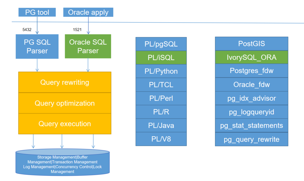
The yellow color in the diagram shows the new modules added by IvorySQL on top of existing PostgreSQL while IvorySQL has also made changes to existing modules and logical structures as well.
The most noteworthy of those modules that received updates for supporting oracle compatibility are backend parser and system catalogs.
2. Database Modeling
2.1. Creating a Database
The first test to see whether you can access the database server is to try to create a database. A running IvorySQL server can manage many databases. Typically, a separate database is used for each project or for each user.
Possibly, your site administrator has already created a database for your use. In that case you can omit this step and skip ahead to the next section.
To create a new database, in this example named mydb, you use the following command:
$ createdb mydbIf this produces no response then this step was successful and you can skip over the remainder of this section.
If you see a message similar to:
createdb: command not foundthen IvorySQL was not installed properly. Either it was not installed at all or your shell’s search path was not set to include it. Try calling the command with an absolute path instead:
$ /usr/local/pgsql/bin/createdb mydbThe path at your site might be different. Contact your site administrator or check the installation instructions to correct the situation.
Another response could be this:
createdb: error: connection to server on socket "/tmp/.s.PGSQL.5432" failed: No such file or directory
        Is the server running locally and accepting connections on that socket?
This means that the server was not started, or it is not listening where createdb expects to contact it. Again, check the installation instructions or consult the administrator.
Another response could be this:
createdb: error: connection to server on socket "/tmp/.s.PGSQL.5432" failed: FATAL: role "joe" does not existwhere your own login name is mentioned. This will happen if the administrator has not created a IvorySQL user account for you. (IvorySQL user accounts are distinct from operating system user accounts.) If you are the administrator, You will need to become the operating system user under which IvorySQL was installed (usually postgres) to create the first user account. It could also be that you were assigned a IvorySQL user name that is different from your operating system user name; in that case you need to use the -U switch or set the PGUSER environment variable to specify your IvorySQL user name.
If you have a user account but it does not have the privileges required to create a database, you will see the following:
createdb: error: database creation failed: ERROR: permission denied to create databaseNot every user has authorization to create new databases. If IvorySQL refuses to create databases for you then the site administrator needs to grant you permission to create databases. Consult your site administrator if this occurs. If you installed IvorySQL yourself then you should log in for the purposes of this tutorial under the user account that you started the server as. [1]
You can also create databases with other names. IvorySQL allows you to create any number of databases at a given site. Database names must have an alphabetic first character and are limited to 63 bytes in length. A convenient choice is to create a database with the same name as your current user name. Many tools assume that database name as the default, so it can save you some typing. To create that database, simply type:
$ createdbIf you do not want to use your database anymore you can remove it. For example, if you are the owner (creator) of the database mydb, you can destroy it using the following command:
$ dropdb mydb(For this command, the database name does not default to the user account name. You always need to specify it.) This action physically removes all files associated with the database and cannot be undone, so this should only be done with a great deal of forethought.
2.2. Creating a New Table
You can create a new table by specifying the table name, along with all column names and their types:
CREATE TABLE weather (
    city            varchar(80),
    temp_lo         int,           -- low temperature
    temp_hi         int,           -- high temperature
    prcp            real,          -- precipitation
    date            date
);
You can enter this into psql with the line breaks. psql will recognize that the command is not terminated until the semicolon.
White space (i.e., spaces, tabs, and newlines) can be used freely in SQL commands. That means you can type the command aligned differently than above, or even all on one line. Two dashes (“--”) introduce comments. Whatever follows them is ignored up to the end of the line. SQL is case insensitive about key words and identifiers, except when identifiers are double-quoted to preserve the case (not done above).
varchar(80) specifies a data type that can store arbitrary character strings up to 80 characters in length. int is the normal integer type. real is a type for storing single precision floating-point numbers. date should be self-explanatory. (Yes, the column of type date is also named date. This might be convenient or confusing — you choose.)
IvorySQL supports the standard SQL types int, smallint, real, double precision, char(`N), `varchar(`N), `date, time, timestamp, and interval, as well as other types of general utility and a rich set of geometric types. IvorySQL can be customized with an arbitrary number of user-defined data types. Consequently, type names are not key words in the syntax, except where required to support special cases in the SQL standard.
The second example will store cities and their associated geographical location:
CREATE TABLE cities (
    name            varchar(80),
    location        point
);
The point type is an example of a IvorySQL-specific data type.
Finally, it should be mentioned that if you don’t need a table any longer or want to recreate it differently you can remove it using the following command:
DROP TABLE tablename;3. Write to data
When a table is created, it contains no data. The first thing to do before a database can be of much use is to insert data. Data is inserted one row at a time. You can also insert more than one row in a single command, but it is not possible to insert something that is not a complete row. Even if you know only some column values, a complete row must be created.
To create a new row, use the INSERT command. The command requires the table name and column values.
CREATE TABLE products (
    product_no integer,
    name text,
    price numeric
);
An example command to insert a row would be:
INSERT INTO products VALUES (1, 'Cheese', 9.99);The data values are listed in the order in which the columns appear in the table, separated by commas. Usually, the data values will be literals (constants), but scalar expressions are also allowed.
The above syntax has the drawback that you need to know the order of the columns in the table. To avoid this you can also list the columns explicitly. For example, both of the following commands have the same effect as the one above:
INSERT INTO products (product_no, name, price) VALUES (1, 'Cheese', 9.99);
INSERT INTO products (name, price, product_no) VALUES ('Cheese', 9.99, 1);
Many users consider it good practice to always list the column names.
If you don’t have values for all the columns, you can omit some of them. In that case, the columns will be filled with their default values. For example:
INSERT INTO products (product_no, name) VALUES (1, 'Cheese');
INSERT INTO products VALUES (1, 'Cheese');
The second form is a IvorySQL extension. It fills the columns from the left with as many values as are given, and the rest will be defaulted.
For clarity, you can also request default values explicitly, for individual columns or for the entire row:
INSERT INTO products (product_no, name, price) VALUES (1, 'Cheese', DEFAULT);
INSERT INTO products DEFAULT VALUES;
You can insert multiple rows in a single command:
INSERT INTO products (product_no, name, price) VALUES
    (1, 'Cheese', 9.99),
    (2, 'Bread', 1.99),
    (3, 'Milk', 2.99);
It is also possible to insert the result of a query (which might be no rows, one row, or many rows):
INSERT INTO products (product_no, name, price)
  SELECT product_no, name, price FROM new_products
    WHERE release_date = 'today';
This provides the full power of the SQL query mechanism for computing the rows to be inserted.
4. Query Data
4.1. Combining Queries (UNION, INTERSECT, EXCEPT)
The results of two queries can be combined using the set operations union, intersection, and difference. The syntax is
query1 UNION [ALL] query2
query1 INTERSECT [ALL] query2
query1 EXCEPT [ALL] query2
where query1 and query2 are queries that can use any of the features discussed up to this point.
UNION effectively appends the result of query2 to the result of query1 (although there is no guarantee that this is the order in which the rows are actually returned). Furthermore, it eliminates duplicate rows from its result, in the same way as DISTINCT, unless UNION ALL is used.
INTERSECT returns all rows that are both in the result of query1 and in the result of query2. Duplicate rows are eliminated unless INTERSECT ALL is used.
EXCEPT returns all rows that are in the result of query1 but not in the result of query2. (This is sometimes called the difference between two queries.) Again, duplicates are eliminated unless EXCEPT ALL is used.
In order to calculate the union, intersection, or difference of two queries, the two queries must be “union compatible”, which means that they return the same number of columns and the corresponding columns have compatible data types.
Set operations can be combined, for example
query1 UNION query2 EXCEPT query3which is equivalent to
(query1 UNION query2) EXCEPT query3As shown here, you can use parentheses to control the order of evaluation. Without parentheses, UNION and EXCEPT associate left-to-right, but INTERSECT binds more tightly than those two operators. Thus
query1 UNION query2 INTERSECT query3means
query1 UNION (query2 INTERSECT query3)You can also surround an individual query with parentheses. This is important if the query needs to use any of the clauses discussed in following sections, such as LIMIT. Without parentheses, you’ll get a syntax error, or else the clause will be understood as applying to the output of the set operation rather than one of its inputs. For example,
SELECT a FROM b UNION SELECT x FROM y LIMIT 10is accepted, but it means
(SELECT a FROM b UNION SELECT x FROM y) LIMIT 10not
SELECT a FROM b UNION (SELECT x FROM y LIMIT 10)4.2. Parallel Query
4.2.1. How Parallel Query Works
When the optimizer determines that parallel query is the fastest execution strategy for a particular query, it will create a query plan that includes a Gather or Gather Merge node. Here is a simple example:
EXPLAIN SELECT * FROM pgbench_accounts WHERE filler LIKE '%x%';
                                     QUERY PLAN
-------------------------------------------------------------------------------------
 Gather  (cost=1000.00..217018.43 rows=1 width=97)
   Workers Planned: 2
   ->  Parallel Seq Scan on pgbench_accounts  (cost=0.00..216018.33 rows=1 width=97)
         Filter: (filler ~~ '%x%'::text)
(4 rows)
In all cases, the Gather or Gather Merge node will have exactly one child plan, which is the portion of the plan that will be executed in parallel. If the Gather or Gather Merge node is at the very top of the plan tree, then the entire query will execute in parallel. If it is somewhere else in the plan tree, then only the portion of the plan below it will run in parallel. In the example above, the query accesses only one table, so there is only one plan node other than the Gather node itself; since that plan node is a child of the Gather node, it will run in parallel.
Using EXPLAIN, you can see the number of workers chosen by the planner. When the Gather node is reached during query execution, the process that is implementing the user’s session will request a number of background worker processes equal to the number of workers chosen by the planner. The number of background workers that the planner will consider using is limited to at most max_parallel_workers_per_gather. The total number of background workers that can exist at any one time is limited by both max_worker_processes and max_parallel_workers. Therefore, it is possible for a parallel query to run with fewer workers than planned, or even with no workers at all. The optimal plan may depend on the number of workers that are available, so this can result in poor query performance. If this occurrence is frequent, consider increasing max_worker_processes and max_parallel_workers so that more workers can be run simultaneously or alternatively reducing max_parallel_workers_per_gather so that the planner requests fewer workers.
Every background worker process that is successfully started for a given parallel query will execute the parallel portion of the plan. The leader will also execute that portion of the plan, but it has an additional responsibility: it must also read all of the tuples generated by the workers. When the parallel portion of the plan generates only a small number of tuples, the leader will often behave very much like an additional worker, speeding up query execution. Conversely, when the parallel portion of the plan generates a large number of tuples, the leader may be almost entirely occupied with reading the tuples generated by the workers and performing any further processing steps that are required by plan nodes above the level of the Gather node or Gather Merge node. In such cases, the leader will do very little of the work of executing the parallel portion of the plan.
When the node at the top of the parallel portion of the plan is Gather Merge rather than Gather, it indicates that each process executing the parallel portion of the plan is producing tuples in sorted order, and that the leader is performing an order-preserving merge. In contrast, Gather reads tuples from the workers in whatever order is convenient, destroying any sort order that may have existed.
4.2.2. When Can Parallel Query Be Used?
There are several settings that can cause the query planner not to generate a parallel query plan under any circumstances. In order for any parallel query plans whatsoever to be generated, the following settings must be configured as indicated.
-
max_parallel_workers_per_gather must be set to a value that is greater than zero. This is a special case of the more general principle that no more workers should be used than the number configured via
max_parallel_workers_per_gather.
In addition, the system must not be running in single-user mode. Since the entire database system is running as a single process in this situation, no background workers will be available.
Even when it is in general possible for parallel query plans to be generated, the planner will not generate them for a given query if any of the following are true:
-
The query writes any data or locks any database rows. If a query contains a data-modifying operation either at the top level or within a CTE, no parallel plans for that query will be generated. As an exception, the following commands, which create a new table and populate it, can use a parallel plan for the underlying
SELECTpart of the query: -
CREATE TABLE … AS -
SELECT INTO -
CREATE MATERIALIZED VIEW -
REFRESH MATERIALIZED VIEW -
The query might be suspended during execution. In any situation in which the system thinks that partial or incremental execution might occur, no parallel plan is generated. For example, a cursor created using DECLARE CURSOR will never use a parallel plan. Similarly, a PL/pgSQL loop of the form
FOR x IN query LOOP .. END LOOPwill never use a parallel plan, because the parallel query system is unable to verify that the code in the loop is safe to execute while parallel query is active. -
The query uses any function marked
PARALLEL UNSAFE. Most system-defined functions arePARALLEL SAFE, but user-defined functions are markedPARALLEL UNSAFEby default. -
The query is running inside of another query that is already parallel. For example, if a function called by a parallel query issues an SQL query itself, that query will never use a parallel plan. This is a limitation of the current implementation, but it may not be desirable to remove this limitation, since it could result in a single query using a very large number of processes.
Even when parallel query plan is generated for a particular query, there are several circumstances under which it will be impossible to execute that plan in parallel at execution time. If this occurs, the leader will execute the portion of the plan below the Gather node entirely by itself, almost as if the Gather node were not present. This will happen if any of the following conditions are met:
-
No background workers can be obtained because of the limitation that the total number of background workers cannot exceed max_worker_processes.
-
No background workers can be obtained because of the limitation that the total number of background workers launched for purposes of parallel query cannot exceed max_parallel_workers.
-
The client sends an Execute message with a non-zero fetch count. See the discussion of the extended query protocol. Since libpq currently provides no way to send such a message, this can only occur when using a client that does not rely on libpq. If this is a frequent occurrence, it may be a good idea to set max_parallel_workers_per_gather to zero in sessions where it is likely, so as to avoid generating query plans that may be suboptimal when run serially.
4.2.3. Parallel Plans
Because each worker executes the parallel portion of the plan to completion, it is not possible to simply take an ordinary query plan and run it using multiple workers. Each worker would produce a full copy of the output result set, so the query would not run any faster than normal but would produce incorrect results. Instead, the parallel portion of the plan must be what is known internally to the query optimizer as a partial plan; that is, it must be constructed so that each process that executes the plan will generate only a subset of the output rows in such a way that each required output row is guaranteed to be generated by exactly one of the cooperating processes. Generally, this means that the scan on the driving table of the query must be a parallel-aware scan.
4.2.3.1. Parallel Scans
The following types of parallel-aware table scans are currently supported.
-
In a parallel sequential scan, the table’s blocks will be divided into ranges and shared among the cooperating processes. Each worker process will complete the scanning of its given range of blocks before requesting an additional range of blocks.
-
In a parallel bitmap heap scan, one process is chosen as the leader. That process performs a scan of one or more indexes and builds a bitmap indicating which table blocks need to be visited. These blocks are then divided among the cooperating processes as in a parallel sequential scan. In other words, the heap scan is performed in parallel, but the underlying index scan is not.
-
In a parallel index scan or parallel index-only scan, the cooperating processes take turns reading data from the index. Currently, parallel index scans are supported only for btree indexes. Each process will claim a single index block and will scan and return all tuples referenced by that block; other processes can at the same time be returning tuples from a different index block. The results of a parallel btree scan are returned in sorted order within each worker process.
Other scan types, such as scans of non-btree indexes, may support parallel scans in the future.
4.2.3.2. Parallel Joins
Just as in a non-parallel plan, the driving table may be joined to one or more other tables using a nested loop, hash join, or merge join. The inner side of the join may be any kind of non-parallel plan that is otherwise supported by the planner provided that it is safe to run within a parallel worker. Depending on the join type, the inner side may also be a parallel plan.
-
In a nested loop join, the inner side is always non-parallel. Although it is executed in full, this is efficient if the inner side is an index scan, because the outer tuples and thus the loops that look up values in the index are divided over the cooperating processes.
-
In a merge join, the inner side is always a non-parallel plan and therefore executed in full. This may be inefficient, especially if a sort must be performed, because the work and resulting data are duplicated in every cooperating process.
-
In a hash join (without the "parallel" prefix), the inner side is executed in full by every cooperating process to build identical copies of the hash table. This may be inefficient if the hash table is large or the plan is expensive. In a parallel hash join, the inner side is a parallel hash that divides the work of building a shared hash table over the cooperating processes.
4.2.3.3. Parallel Aggregation
IvorySQL supports parallel aggregation by aggregating in two stages. First, each process participating in the parallel portion of the query performs an aggregation step, producing a partial result for each group of which that process is aware. This is reflected in the plan as a Partial Aggregate node. Second, the partial results are transferred to the leader via Gather or Gather Merge. Finally, the leader re-aggregates the results across all workers in order to produce the final result. This is reflected in the plan as a Finalize Aggregate node.
Because the Finalize Aggregate node runs on the leader process, queries that produce a relatively large number of groups in comparison to the number of input rows will appear less favorable to the query planner. For example, in the worst-case scenario the number of groups seen by the Finalize Aggregate node could be as many as the number of input rows that were seen by all worker processes in the Partial Aggregate stage. For such cases, there is clearly going to be no performance benefit to using parallel aggregation. The query planner takes this into account during the planning process and is unlikely to choose parallel aggregate in this scenario.
Parallel aggregation is not supported in all situations. Each aggregate must be safe for parallelism and must have a combine function. If the aggregate has a transition state of type internal, it must have serialization and deserialization functions. See CREATE AGGREGATE for more details. Parallel aggregation is not supported if any aggregate function call contains DISTINCT or ORDER BY clause and is also not supported for ordered set aggregates or when the query involves GROUPING SETS. It can only be used when all joins involved in the query are also part of the parallel portion of the plan.
4.2.3.4. Parallel Append
Whenever IvorySQL needs to combine rows from multiple sources into a single result set, it uses an Append or MergeAppend plan node. This commonly happens when implementing UNION ALL or when scanning a partitioned table. Such nodes can be used in parallel plans just as they can in any other plan. However, in a parallel plan, the planner may instead use a Parallel Append node.
When an Append node is used in a parallel plan, each process will execute the child plans in the order in which they appear, so that all participating processes cooperate to execute the first child plan until it is complete and then move to the second plan at around the same time. When a Parallel Append is used instead, the executor will instead spread out the participating processes as evenly as possible across its child plans, so that multiple child plans are executed simultaneously. This avoids contention, and also avoids paying the startup cost of a child plan in those processes that never execute it.
Also, unlike a regular Append node, which can only have partial children when used within a parallel plan, a Parallel Append node can have both partial and non-partial child plans. Non-partial children will be scanned by only a single process, since scanning them more than once would produce duplicate results. Plans that involve appending multiple results sets can therefore achieve coarse-grained parallelism even when efficient partial plans are not available. For example, consider a query against a partitioned table that can only be implemented efficiently by using an index that does not support parallel scans. The planner might choose a Parallel Append of regular Index Scan plans; each individual index scan would have to be executed to completion by a single process, but different scans could be performed at the same time by different processes.
enable_parallel_append can be used to disable this feature.
4.2.3.5. Parallel Plan Tips
If a query that is expected to do so does not produce a parallel plan, you can try reducing parallel_setup_cost or parallel_tuple_cost. Of course, this plan may turn out to be slower than the serial plan that the planner preferred, but this will not always be the case. If you don’t get a parallel plan even with very small values of these settings (e.g., after setting them both to zero), there may be some reason why the query planner is unable to generate a parallel plan for your query.
When executing a parallel plan, you can use EXPLAIN (ANALYZE, VERBOSE) to display per-worker statistics for each plan node. This may be useful in determining whether the work is being evenly distributed between all plan nodes and more generally in understanding the performance characteristics of the plan.
5. Transaction
5.1. ABORT — abort the current transaction
5.1.2. Description
ABORT rolls back the current transaction and causes all the updates made by the transaction to be discarded. This command is identical in behavior to the standard SQL command ROLLBACK, and is present only for historical reasons.
5.1.3. Parameters
-
WORKTRANSACTION
Optional key words. They have no effect.
-
AND CHAIN
If AND CHAIN is specified, a new transaction is immediately started with the same transaction characteristics (see SET TRANSACTION) as the just finished one. Otherwise, no new transaction is started.
5.1.4. Notes
Use COMMIT to successfully terminate a transaction.
Issuing ABORT outside of a transaction block emits a warning and otherwise has no effect.
5.2. BEGIN — start a transaction block
5.2.1. Synopsis
BEGIN [ WORK | TRANSACTION ] [ transaction_mode [, ...] ]

where transaction_mode is one of:

    ISOLATION LEVEL { SERIALIZABLE | REPEATABLE READ | READ COMMITTED | READ UNCOMMITTED }
    READ WRITE | READ ONLY
    [ NOT ] DEFERRABLE
5.2.2. Description
BEGIN initiates a transaction block, that is, all statements after a BEGIN command will be executed in a single transaction until an explicit COMMIT or ROLLBACK is given. By default (without BEGIN), IvorySQL executes transactions in “autocommit” mode, that is, each statement is executed in its own transaction and a commit is implicitly performed at the end of the statement (if execution was successful, otherwise a rollback is done).
Statements are executed more quickly in a transaction block, because transaction start/commit requires significant CPU and disk activity. Execution of multiple statements inside a transaction is also useful to ensure consistency when making several related changes: other sessions will be unable to see the intermediate states wherein not all the related updates have been done.
If the isolation level, read/write mode, or deferrable mode is specified, the new transaction has those characteristics, as if SET TRANSACTION was executed.
5.2.3. Parameters
-
WORKTRANSACTION
Optional key words. They have no effect.
Refer to SET TRANSACTION for information on the meaning of the other parameters to this statement.
5.2.4. Notes
START TRANSACTION has the same functionality as BEGIN.
Issuing BEGIN when already inside a transaction block will provoke a warning message. The state of the transaction is not affected. To nest transactions within a transaction block, use savepoints (see SAVEPOINT).
For reasons of backwards compatibility, the commas between successive transaction_modes can be omitted.
5.2.6. Compatibility
BEGIN is a IvorySQL language extension. It is equivalent to the SQL-standard command START TRANSACTION, whose reference page contains additional compatibility information.
The DEFERRABLE transaction_mode is a IvorySQL language extension.
Incidentally, the BEGIN key word is used for a different purpose in embedded SQL. You are advised to be careful about the transaction semantics when porting database applications.
5.3. COMMIT — commit the current transaction
5.3.2. Description
COMMIT commits the current transaction. All changes made by the transaction become visible to others and are guaranteed to be durable if a crash occurs.
5.3.3. Parameters
-
WORKTRANSACTION
Optional key words. They have no effect.
-
AND CHAIN
If AND CHAIN is specified, a new transaction is immediately started with the same transaction characteristics (see SET TRANSACTION) as the just finished one. Otherwise, no new transaction is started.
5.3.4. Notes
Use ROLLBACK to abort a transaction.
Issuing COMMIT when not inside a transaction does no harm, but it will provoke a warning message. COMMIT AND CHAIN when not inside a transaction is an error.
5.4. COMMIT PREPARED — commit a transaction that was earlier prepared for two-phase commit
5.4.3. Parameters
-
transaction_id
The transaction identifier of the transaction that is to be committed.
5.4.4. Notes
To commit a prepared transaction, you must be either the same user that executed the transaction originally, or a superuser. But you do not have to be in the same session that executed the transaction.
This command cannot be executed inside a transaction block. The prepared transaction is committed immediately.
All currently available prepared transactions are listed in the pg_prepared_xacts system view.
5.5. END — commit the current transaction
5.5.2. Description
END commits the current transaction. All changes made by the transaction become visible to others and are guaranteed to be durable if a crash occurs. This command is a IvorySQL extension that is equivalent to COMMIT.
5.5.3. Parameters
-
WORKTRANSACTION
Optional key words. They have no effect.
-
AND CHAIN
If AND CHAIN is specified, a new transaction is immediately started with the same transaction characteristics (see SET TRANSACTION) as the just finished one. Otherwise, no new transaction is started.
5.5.4. Notes
Use ROLLBACK to abort a transaction.
Issuing END when not inside a transaction does no harm, but it will provoke a warning message.
5.5.6. Compatibility
END is a IvorySQL extension that provides functionality equivalent to COMMIT, which is specified in the SQL standard.
5.6. PREPARE TRANSACTION — prepare the current transaction for two-phase commit
5.6.2. Description
PREPARE TRANSACTION prepares the current transaction for two-phase commit. After this command, the transaction is no longer associated with the current session; instead, its state is fully stored on disk, and there is a very high probability that it can be committed successfully, even if a database crash occurs before the commit is requested.
Once prepared, a transaction can later be committed or rolled back with COMMIT PREPARED or ROLLBACK PREPARED, respectively. Those commands can be issued from any session, not only the one that executed the original transaction.
From the point of view of the issuing session, PREPARE TRANSACTION is not unlike a ROLLBACK command: after executing it, there is no active current transaction, and the effects of the prepared transaction are no longer visible. (The effects will become visible again if the transaction is committed.)
If the PREPARE TRANSACTION command fails for any reason, it becomes a ROLLBACK: the current transaction is canceled.
5.6.3. Parameters
-
transaction_id
An arbitrary identifier that later identifies this transaction for COMMIT PREPARED or ROLLBACK PREPARED. The identifier must be written as a string literal, and must be less than 200 bytes long. It must not be the same as the identifier used for any currently prepared transaction.
5.6.4. Notes
PREPARE TRANSACTION is not intended for use in applications or interactive sessions. Its purpose is to allow an external transaction manager to perform atomic global transactions across multiple databases or other transactional resources. Unless you’re writing a transaction manager, you probably shouldn’t be using PREPARE TRANSACTION.
This command must be used inside a transaction block. Use BEGIN to start one.
It is not currently allowed to PREPARE a transaction that has executed any operations involving temporary tables or the session’s temporary namespace, created any cursors WITH HOLD, or executed LISTEN, UNLISTEN, or NOTIFY. Those features are too tightly tied to the current session to be useful in a transaction to be prepared.
If the transaction modified any run-time parameters with SET (without the LOCAL option), those effects persist after PREPARE TRANSACTION, and will not be affected by any later COMMIT PREPARED or ROLLBACK PREPARED. Thus, in this one respect PREPARE TRANSACTION acts more like COMMIT than ROLLBACK.
All currently available prepared transactions are listed in the pg_prepared_xacts system view.
5.6.5. Caution
It is unwise to leave transactions in the prepared state for a long time. This will interfere with the ability of VACUUM to reclaim storage, and in extreme cases could cause the database to shut down to prevent transaction ID wraparound (see Section 25.1.5). Keep in mind also that the transaction continues to hold whatever locks it held. The intended usage of the feature is that a prepared transaction will normally be committed or rolled back as soon as an external transaction manager has verified that other databases are also prepared to commit.
If you have not set up an external transaction manager to track prepared transactions and ensure they get closed out promptly, it is best to keep the prepared-transaction feature disabled by setting max_prepared_transactions to zero. This will prevent accidental creation of prepared transactions that might then be forgotten and eventually cause problems.
5.7. ROLLBACK — abort the current transaction
5.7.2. Description
ROLLBACK rolls back the current transaction and causes all the updates made by the transaction to be discarded.
5.7.3. Parameters
-
WORKTRANSACTION
Optional key words. They have no effect.
-
AND CHAIN
If AND CHAIN is specified, a new transaction is immediately started with the same transaction characteristics (see SET TRANSACTION) as the just finished one. Otherwise, no new transaction is started.
5.7.4. Notes
Use COMMIT to successfully terminate a transaction.
Issuing ROLLBACK outside of a transaction block emits a warning and otherwise has no effect. ROLLBACK AND CHAIN outside of a transaction block is an error.
5.8. ROLLBACK PREPARED — cancel a transaction that was earlier prepared for two-phase commit
5.8.3. Parameters
-
transaction_id
The transaction identifier of the transaction that is to be rolled back.
5.8.4. Notes
To roll back a prepared transaction, you must be either the same user that executed the transaction originally, or a superuser. But you do not have to be in the same session that executed the transaction.
This command cannot be executed inside a transaction block. The prepared transaction is rolled back immediately.
All currently available prepared transactions are listed in the pg_prepared_xacts system view.
5.9. SAVEPOINT — define a new savepoint within the current transaction
5.9.2. Description
SAVEPOINT establishes a new savepoint within the current transaction.
A savepoint is a special mark inside a transaction that allows all commands that are executed after it was established to be rolled back, restoring the transaction state to what it was at the time of the savepoint.
5.9.3. Parameters
-
savepoint_name
The name to give to the new savepoint. If savepoints with the same name already exist, they will be inaccessible until newer identically-named savepoints are released.
5.9.4. Notes
Use ROLLBACK TO to rollback to a savepoint. Use RELEASE SAVEPOINT to destroy a savepoint, keeping the effects of commands executed after it was established.
Savepoints can only be established when inside a transaction block. There can be multiple savepoints defined within a transaction.
5.9.5. Examples
To establish a savepoint and later undo the effects of all commands executed after it was established:
BEGIN;
    INSERT INTO table1 VALUES (1);
    SAVEPOINT my_savepoint;
    INSERT INTO table1 VALUES (2);
    ROLLBACK TO SAVEPOINT my_savepoint;
    INSERT INTO table1 VALUES (3);
COMMIT;
The above transaction will insert the values 1 and 3, but not 2.
To establish and later destroy a savepoint:
BEGIN;
    INSERT INTO table1 VALUES (3);
    SAVEPOINT my_savepoint;
    INSERT INTO table1 VALUES (4);
    RELEASE SAVEPOINT my_savepoint;
COMMIT;
The above transaction will insert both 3 and 4.
To use a single savepoint name:
BEGIN;
    INSERT INTO table1 VALUES (1);
    SAVEPOINT my_savepoint;
    INSERT INTO table1 VALUES (2);
    SAVEPOINT my_savepoint;
    INSERT INTO table1 VALUES (3);

    -- rollback to the second savepoint
    ROLLBACK TO SAVEPOINT my_savepoint;
    SELECT * FROM table1;               -- shows rows 1 and 2

    -- release the second savepoint
    RELEASE SAVEPOINT my_savepoint;

    -- rollback to the first savepoint
    ROLLBACK TO SAVEPOINT my_savepoint;
    SELECT * FROM table1;               -- shows only row 1
COMMIT;
The above transaction shows row 3 being rolled back first, then row 2.
5.9.6. Compatibility
SQL requires a savepoint to be destroyed automatically when another savepoint with the same name is established. In IvorySQL, the old savepoint is kept, though only the more recent one will be used when rolling back or releasing. (Releasing the newer savepoint with RELEASE SAVEPOINT will cause the older one to again become accessible to ROLLBACK TO SAVEPOINT and RELEASE SAVEPOINT.) Otherwise, SAVEPOINT is fully SQL conforming.
5.10. SET CONSTRAINTS — set constraint check timing for the current transaction
5.10.2. Description
SET CONSTRAINTS sets the behavior of constraint checking within the current transaction. IMMEDIATE constraints are checked at the end of each statement. DEFERRED constraints are not checked until transaction commit. Each constraint has its own IMMEDIATE or DEFERRED mode.
Upon creation, a constraint is given one of three characteristics: DEFERRABLE INITIALLY DEFERRED, DEFERRABLE INITIALLY IMMEDIATE, or NOT DEFERRABLE. The third class is always IMMEDIATE and is not affected by the SET CONSTRAINTS command. The first two classes start every transaction in the indicated mode, but their behavior can be changed within a transaction by SET CONSTRAINTS.
SET CONSTRAINTS with a list of constraint names changes the mode of just those constraints (which must all be deferrable). Each constraint name can be schema-qualified. The current schema search path is used to find the first matching name if no schema name is specified. SET CONSTRAINTS ALL changes the mode of all deferrable constraints.
When SET CONSTRAINTS changes the mode of a constraint from DEFERRED to IMMEDIATE, the new mode takes effect retroactively: any outstanding data modifications that would have been checked at the end of the transaction are instead checked during the execution of the SET CONSTRAINTS command. If any such constraint is violated, the SET CONSTRAINTS fails (and does not change the constraint mode). Thus, SET CONSTRAINTS can be used to force checking of constraints to occur at a specific point in a transaction.
Currently, only UNIQUE, PRIMARY KEY, REFERENCES (foreign key), and EXCLUDE constraints are affected by this setting. NOT NULL and CHECK constraints are always checked immediately when a row is inserted or modified (not at the end of the statement). Uniqueness and exclusion constraints that have not been declared DEFERRABLE are also checked immediately.
The firing of triggers that are declared as “constraint triggers” is also controlled by this setting — they fire at the same time that the associated constraint should be checked.
5.10.3. Notes
Because IvorySQL does not require constraint names to be unique within a schema (but only per-table), it is possible that there is more than one match for a specified constraint name. In this case SET CONSTRAINTS will act on all matches. For a non-schema-qualified name, once a match or matches have been found in some schema in the search path, schemas appearing later in the path are not searched.
This command only alters the behavior of constraints within the current transaction. Issuing this outside of a transaction block emits a warning and otherwise has no effect.
5.10.4. Compatibility
This command complies with the behavior defined in the SQL standard, except for the limitation that, in IvorySQL, it does not apply to NOT NULL and CHECK constraints. Also, IvorySQL checks non-deferrable uniqueness constraints immediately, not at end of statement as the standard would suggest.
5.11. SET TRANSACTION — set the characteristics of the current transaction
5.11.1. Synopsis
SET TRANSACTION transaction_mode [, ...]
SET TRANSACTION SNAPSHOT snapshot_id
SET SESSION CHARACTERISTICS AS TRANSACTION transaction_mode [, ...]

where transaction_mode is one of:

    ISOLATION LEVEL { SERIALIZABLE | REPEATABLE READ | READ COMMITTED | READ UNCOMMITTED }
    READ WRITE | READ ONLY
    [ NOT ] DEFERRABLE
5.11.2. Description
The SET TRANSACTION command sets the characteristics of the current transaction. It has no effect on any subsequent transactions. SET SESSION CHARACTERISTICS sets the default transaction characteristics for subsequent transactions of a session. These defaults can be overridden by SET TRANSACTION for an individual transaction.
The available transaction characteristics are the transaction isolation level, the transaction access mode (read/write or read-only), and the deferrable mode. In addition, a snapshot can be selected, though only for the current transaction, not as a session default.
The isolation level of a transaction determines what data the transaction can see when other transactions are running concurrently:
-
READ COMMITTED
A statement can only see rows committed before it began. This is the default.
-
REPEATABLE READ
All statements of the current transaction can only see rows committed before the first query or data-modification statement was executed in this transaction.
-
SERIALIZABLE
All statements of the current transaction can only see rows committed before the first query or data-modification statement was executed in this transaction. If a pattern of reads and writes among concurrent serializable transactions would create a situation which could not have occurred for any serial (one-at-a-time) execution of those transactions, one of them will be rolled back with a serialization_failure error.
The SQL standard defines one additional level, READ UNCOMMITTED. In IvorySQL READ UNCOMMITTED is treated as READ COMMITTED.
The transaction isolation level cannot be changed after the first query or data-modification statement (SELECT, INSERT, DELETE, UPDATE, FETCH, or COPY) of a transaction has been executed. See Chapter 13 for more information about transaction isolation and concurrency control.
The transaction access mode determines whether the transaction is read/write or read-only. Read/write is the default. When a transaction is read-only, the following SQL commands are disallowed: INSERT, UPDATE, DELETE, and COPY FROM if the table they would write to is not a temporary table; all CREATE, ALTER, and DROP commands; COMMENT, GRANT, REVOKE, TRUNCATE; and EXPLAIN ANALYZE and EXECUTE if the command they would execute is among those listed. This is a high-level notion of read-only that does not prevent all writes to disk.
The DEFERRABLE transaction property has no effect unless the transaction is also SERIALIZABLE and READ ONLY. When all three of these properties are selected for a transaction, the transaction may block when first acquiring its snapshot, after which it is able to run without the normal overhead of a SERIALIZABLE transaction and without any risk of contributing to or being canceled by a serialization failure. This mode is well suited for long-running reports or backups.
The SET TRANSACTION SNAPSHOT command allows a new transaction to run with the same snapshot as an existing transaction. The pre-existing transaction must have exported its snapshot with the pg_export_snapshot function. That function returns a snapshot identifier, which must be given to SET TRANSACTION SNAPSHOT to specify which snapshot is to be imported. The identifier must be written as a string literal in this command, for example '00000003-0000001B-1'. SET TRANSACTION SNAPSHOT can only be executed at the start of a transaction, before the first query or data-modification statement (SELECT, INSERT, DELETE, UPDATE, FETCH, or COPY) of the transaction. Furthermore, the transaction must already be set to SERIALIZABLE or REPEATABLE READ isolation level (otherwise, the snapshot would be discarded immediately, since READ COMMITTED mode takes a new snapshot for each command). If the importing transaction uses SERIALIZABLE isolation level, then the transaction that exported the snapshot must also use that isolation level. Also, a non-read-only serializable transaction cannot import a snapshot from a read-only transaction.
5.11.3. Notes
If SET TRANSACTION is executed without a prior START TRANSACTION or BEGIN, it emits a warning and otherwise has no effect.
It is possible to dispense with SET TRANSACTION by instead specifying the desired transaction_modes in BEGIN or START TRANSACTION. But that option is not available for SET TRANSACTION SNAPSHOT.
The session default transaction modes can also be set or examined via the configuration parameters default_transaction_isolation, default_transaction_read_only, and default_transaction_deferrable. (In fact SET SESSION CHARACTERISTICS is just a verbose equivalent for setting these variables with SET.) This means the defaults can be set in the configuration file, via ALTER DATABASE, etc. Consult Chapter 20 for more information.
The current transaction’s modes can similarly be set or examined via the configuration parameters transaction_isolation, transaction_read_only, and transaction_deferrable. Setting one of these parameters acts the same as the corresponding SET TRANSACTION option, with the same restrictions on when it can be done. However, these parameters cannot be set in the configuration file, or from any source other than live SQL.
5.11.4. Examples
To begin a new transaction with the same snapshot as an already existing transaction, first export the snapshot from the existing transaction. That will return the snapshot identifier, for example:
BEGIN TRANSACTION ISOLATION LEVEL REPEATABLE READ;
SELECT pg_export_snapshot();
 pg_export_snapshot
---------------------
 00000003-0000001B-1
(1 row)
Then give the snapshot identifier in a SET TRANSACTION SNAPSHOT command at the beginning of the newly opened transaction:
BEGIN TRANSACTION ISOLATION LEVEL REPEATABLE READ;
SET TRANSACTION SNAPSHOT '00000003-0000001B-1';
5.11.5. Compatibility
These commands are defined in the SQL standard, except for the DEFERRABLE transaction mode and the SET TRANSACTION SNAPSHOT form, which are IvorySQL extensions.
SERIALIZABLE is the default transaction isolation level in the standard. In IvorySQL the default is ordinarily READ COMMITTED, but you can change it as mentioned above.
In the SQL standard, there is one other transaction characteristic that can be set with these commands: the size of the diagnostics area. This concept is specific to embedded SQL, and therefore is not implemented in the IvorySQL server.
The SQL standard requires commas between successive transaction_modes, but for historical reasons IvorySQL allows the commas to be omitted.
5.12. START TRANSACTION — start a transaction block
5.12.1. Synopsis
START TRANSACTION [ transaction_mode [, ...] ]

where transaction_mode is one of:

    ISOLATION LEVEL { SERIALIZABLE | REPEATABLE READ | READ COMMITTED | READ UNCOMMITTED }
    READ WRITE | READ ONLY
    [ NOT ] DEFERRABLE
5.12.2. Description
This command begins a new transaction block. If the isolation level, read/write mode, or deferrable mode is specified, the new transaction has those characteristics, as if SET TRANSACTION was executed. This is the same as the BEGIN command.
5.12.3. Parameters
Refer to SET TRANSACTION for information on the meaning of the parameters to this statement.
5.12.4. Compatibility
In the standard, it is not necessary to issue START TRANSACTION to start a transaction block: any SQL command implicitly begins a block. IvorySQL’s behavior can be seen as implicitly issuing a COMMIT after each command that does not follow START TRANSACTION (or BEGIN), and it is therefore often called “autocommit”. Other relational database systems might offer an autocommit feature as a convenience.
The DEFERRABLE transaction_mode is a IvorySQL language extension.
The SQL standard requires commas between successive transaction_modes, but for historical reasons IvorySQL allows the commas to be omitted.
See also the compatibility section of SET TRANSACTION.
6. Sql Reference
6.1. Lexical Structure
SQL input consists of a sequence of commands. A command is composed of a sequence of tokens, terminated by a semicolon (“;”). The end of the input stream also terminates a command. Which tokens are valid depends on the syntax of the particular command.
A token can be a key word, an identifier, a quoted identifier, a literal (or constant), or a special character symbol. Tokens are normally separated by whitespace (space, tab, newline), but need not be if there is no ambiguity (which is generally only the case if a special character is adjacent to some other token type).
For example, the following is (syntactically) valid SQL input:
SELECT * FROM MY_TABLE;
UPDATE MY_TABLE SET A = 5;
INSERT INTO MY_TABLE VALUES (3, 'hi there');
This is a sequence of three commands, one per line (although this is not required; more than one command can be on a line, and commands can usefully be split across lines).
Additionally, comments can occur in SQL input. They are not tokens, they are effectively equivalent to whitespace.
The SQL syntax is not very consistent regarding what tokens identify commands and which are operands or parameters. The first few tokens are generally the command name, so in the above example we would usually speak of a “SELECT”, an “UPDATE”, and an “INSERT” command. But for instance the UPDATE command always requires a SET token to appear in a certain position, and this particular variation of INSERT also requires a VALUES in order to be complete.
6.1.1. Identifiers and Key Words
Tokens such as SELECT, UPDATE, or VALUES in the example above are examples of key words, that is, words that have a fixed meaning in the SQL language. The tokens MY_TABLE and A are examples of identifiers. They identify names of tables, columns, or other database objects, depending on the command they are used in. Therefore they are sometimes simply called “names”. Key words and identifiers have the same lexical structure, meaning that one cannot know whether a token is an identifier or a key word without knowing the language. A complete list of key words can be found in Appendix C.
SQL identifiers and key words must begin with a letter (a-z, but also letters with diacritical marks and non-Latin letters) or an underscore (_). Subsequent characters in an identifier or key word can be letters, underscores, digits (0-9), or dollar signs ($). Note that dollar signs are not allowed in identifiers according to the letter of the SQL standard, so their use might render applications less portable. The SQL standard will not define a key word that contains digits or starts or ends with an underscore, so identifiers of this form are safe against possible conflict with future extensions of the standard.
The system uses no more than NAMEDATALEN-1 bytes of an identifier; longer names can be written in commands, but they will be truncated. By default, NAMEDATALEN is 64 so the maximum identifier length is 63 bytes. If this limit is problematic, it can be raised by changing the NAMEDATALEN constant in src/include/pg_config_manual.h.
Key words and unquoted identifiers are case insensitive. Therefore:
UPDATE MY_TABLE SET A = 5;can equivalently be written as:
uPDaTE my_TabLE SeT a = 5;A convention often used is to write key words in upper case and names in lower case, e.g.:
UPDATE my_table SET a = 5;There is a second kind of identifier: the delimited identifier or quoted identifier. It is formed by enclosing an arbitrary sequence of characters in double-quotes ("). A delimited identifier is always an identifier, never a key word. So "select" could be used to refer to a column or table named “select”, whereas an unquoted select would be taken as a key word and would therefore provoke a parse error when used where a table or column name is expected. The example can be written with quoted identifiers like this:
UPDATE "my_table" SET "a" = 5;Quoted identifiers can contain any character, except the character with code zero. (To include a double quote, write two double quotes.) This allows constructing table or column names that would otherwise not be possible, such as ones containing spaces or ampersands. The length limitation still applies.
Quoting an identifier also makes it case-sensitive, whereas unquoted names are always folded to lower case. For example, the identifiers FOO, foo, and "foo" are considered the same by IvorySQL, but "Foo" and "FOO" are different from these three and each other. (The folding of unquoted names to lower case in IvorySQL is incompatible with the SQL standard, which says that unquoted names should be folded to upper case. Thus, foo should be equivalent to "FOO" not "foo" according to the standard. If you want to write portable applications you are advised to always quote a particular name or never quote it.)
A variant of quoted identifiers allows including escaped Unicode characters identified by their code points. This variant starts with U& (upper or lower case U followed by ampersand) immediately before the opening double quote, without any spaces in between, for example U&"foo". (Note that this creates an ambiguity with the operator &. Use spaces around the operator to avoid this problem.) Inside the quotes, Unicode characters can be specified in escaped form by writing a backslash followed by the four-digit hexadecimal code point number or alternatively a backslash followed by a plus sign followed by a six-digit hexadecimal code point number. For example, the identifier "data" could be written as
U&"d\0061t\+000061"The following less trivial example writes the Russian word “slon” (elephant) in Cyrillic letters:
U&"\0441\043B\043E\043D"If a different escape character than backslash is desired, it can be specified using the UESCAPE clause after the string, for example:
U&"d!0061t!+000061" UESCAPE '!'The escape character can be any single character other than a hexadecimal digit, the plus sign, a single quote, a double quote, or a whitespace character. Note that the escape character is written in single quotes, not double quotes, after UESCAPE.
To include the escape character in the identifier literally, write it twice.
Either the 4-digit or the 6-digit escape form can be used to specify UTF-16 surrogate pairs to compose characters with code points larger than U+FFFF, although the availability of the 6-digit form technically makes this unnecessary. (Surrogate pairs are not stored directly, but are combined into a single code point.)
If the server encoding is not UTF-8, the Unicode code point identified by one of these escape sequences is converted to the actual server encoding; an error is reported if that’s not possible.
6.1.2. Constants
There are three kinds of implicitly-typed constants in IvorySQL: strings, bit strings, and numbers. Constants can also be specified with explicit types, which can enable more accurate representation and more efficient handling by the system. These alternatives are discussed in the following subsections.
6.1.2.1. String Constants
A string constant in SQL is an arbitrary sequence of characters bounded by single quotes ('), for example 'This is a string'. To include a single-quote character within a string constant, write two adjacent single quotes, e.g., 'Dianne''s horse'. Note that this is not the same as a double-quote character (").
Two string constants that are only separated by whitespace with at least one newline are concatenated and effectively treated as if the string had been written as one constant. For example:
SELECT 'foo'
'bar';
is equivalent to:
SELECT 'foobar';but:
SELECT 'foo' 'bar';is not valid syntax. (This slightly bizarre behavior is specified by SQL; IvorySQL is following the standard.)
6.1.2.2. String Constants With C-Style Escapes
IvorySQL also accepts “escape” string constants, which are an extension to the SQL standard. An escape string constant is specified by writing the letter E (upper or lower case) just before the opening single quote, e.g., E’foo'. (When continuing an escape string constant across lines, write E only before the first opening quote.) Within an escape string, a backslash character (\) begins a C-like backslash escape sequence, in which the combination of backslash and following character(s) represent a special byte value.
Table 5.1. Backslash Escape Sequences
Backslash Escape Sequence |
Interpretation |
|
backspace |
|
form feed |
|
newline |
|
carriage return |
|
tab |
|
octal byte value |
|
hexadecimal byte value |
|
16 or 32-bit hexadecimal Unicode character value |
Any other character following a backslash is taken literally. Thus, to include a backslash character, write two backslashes (\\). Also, a single quote can be included in an escape string by writing \', in addition to the normal way of ''.
It is your responsibility that the byte sequences you create, especially when using the octal or hexadecimal escapes, compose valid characters in the server character set encoding. A useful alternative is to use Unicode escapes or the alternative Unicode escape syntax, ; then the server will check that the character conversion is possible.
6.1.2.3. String Constants With Unicode Escapes
IvorySQL also supports another type of escape syntax for strings that allows specifying arbitrary Unicode characters by code point. A Unicode escape string constant starts with U& (upper or lower case letter U followed by ampersand) immediately before the opening quote, without any spaces in between, for example U&'foo'. (Note that this creates an ambiguity with the operator &. Use spaces around the operator to avoid this problem.) Inside the quotes, Unicode characters can be specified in escaped form by writing a backslash followed by the four-digit hexadecimal code point number or alternatively a backslash followed by a plus sign followed by a six-digit hexadecimal code point number. For example, the string 'data' could be written as
U&'d\0061t\+000061'The following less trivial example writes the Russian word “slon” (elephant) in Cyrillic letters:
U&'\0441\043B\043E\043D'If a different escape character than backslash is desired, it can be specified using the UESCAPE clause after the string, for example:
U&'d!0061t!+000061' UESCAPE '!'The escape character can be any single character other than a hexadecimal digit, the plus sign, a single quote, a double quote, or a whitespace character.
To include the escape character in the string literally, write it twice.
Either the 4-digit or the 6-digit escape form can be used to specify UTF-16 surrogate pairs to compose characters with code points larger than U+FFFF, although the availability of the 6-digit form technically makes this unnecessary. (Surrogate pairs are not stored directly, but are combined into a single code point.)
If the server encoding is not UTF-8, the Unicode code point identified by one of these escape sequences is converted to the actual server encoding; an error is reported if that’s not possible.
Also, the Unicode escape syntax for string constants only works when the configuration parameter standard_conforming_strings is turned on. This is because otherwise this syntax could confuse clients that parse the SQL statements to the point that it could lead to SQL injections and similar security issues. If the parameter is set to off, this syntax will be rejected with an error message.
6.1.2.4. Dollar-Quoted String Constants
While the standard syntax for specifying string constants is usually convenient, it can be difficult to understand when the desired string contains many single quotes or backslashes, since each of those must be doubled. To allow more readable queries in such situations, IvorySQL provides another way, called “dollar quoting”, to write string constants. A dollar-quoted string constant consists of a dollar sign ($), an optional “tag” of zero or more characters, another dollar sign, an arbitrary sequence of characters that makes up the string content, a dollar sign, the same tag that began this dollar quote, and a dollar sign. For example, here are two different ways to specify the string “Dianne’s horse” using dollar quoting:
$$Dianne's horse$$
$SomeTag$Dianne's horse$SomeTag$
Notice that inside the dollar-quoted string, single quotes can be used without needing to be escaped. Indeed, no characters inside a dollar-quoted string are ever escaped: the string content is always written literally. Backslashes are not special, and neither are dollar signs, unless they are part of a sequence matching the opening tag.
It is possible to nest dollar-quoted string constants by choosing different tags at each nesting level. This is most commonly used in writing function definitions. For example:
$function$
BEGIN
    RETURN ($1 ~ $q$[\t\r\n\v\\]$q$);
END;
$function$
Here, the sequence $q$[\t\r\n\v\\]$q$ represents a dollar-quoted literal string [\t\r\n\v\\], which will be recognized when the function body is executed by IvorySQL. But since the sequence does not match the outer dollar quoting delimiter $function$, it is just some more characters within the constant so far as the outer string is concerned.
The tag, if any, of a dollar-quoted string follows the same rules as an unquoted identifier, except that it cannot contain a dollar sign. Tags are case sensitive, so $tag$String content$tag$ is correct, but $TAG$String content$tag$ is not.
A dollar-quoted string that follows a keyword or identifier must be separated from it by whitespace; otherwise the dollar quoting delimiter would be taken as part of the preceding identifier.
Dollar quoting is not part of the SQL standard, but it is often a more convenient way to write complicated string literals than the standard-compliant single quote syntax. It is particularly useful when representing string constants inside other constants, as is often needed in procedural function definitions. With single-quote syntax, each backslash in the above example would have to be written as four backslashes, which would be reduced to two backslashes in parsing the original string constant, and then to one when the inner string constant is re-parsed during function execution.
6.1.2.5. Bit-String Constants
Bit-string constants look like regular string constants with a B (upper or lower case) immediately before the opening quote (no intervening whitespace), e.g., B'1001'. The only characters allowed within bit-string constants are 0 and 1.
Alternatively, bit-string constants can be specified in hexadecimal notation, using a leading X (upper or lower case), e.g., X'1FF'. This notation is equivalent to a bit-string constant with four binary digits for each hexadecimal digit.
Both forms of bit-string constant can be continued across lines in the same way as regular string constants. Dollar quoting cannot be used in a bit-string constant.
6.1.2.6. Numeric Constants
Numeric constants are accepted in these general forms:
digits
digits.[digits][e[+-]digits]
[digits].digits[e[+-]digits]
digitse[+-]digits
where digits is one or more decimal digits (0 through 9). At least one digit must be before or after the decimal point, if one is used. At least one digit must follow the exponent marker (e), if one is present. There cannot be any spaces or other characters embedded in the constant. Note that any leading plus or minus sign is not actually considered part of the constant; it is an operator applied to the constant.
These are some examples of valid numeric constants:
A numeric constant that contains neither a decimal point nor an exponent is initially presumed to be type integer if its value fits in type integer (32 bits); otherwise it is presumed to be type bigint if its value fits in type bigint (64 bits); otherwise it is taken to be type numeric. Constants that contain decimal points and/or exponents are always initially presumed to be type numeric.
The initially assigned data type of a numeric constant is just a starting point for the type resolution algorithms. In most cases the constant will be automatically coerced to the most appropriate type depending on context. When necessary, you can force a numeric value to be interpreted as a specific data type by casting it. For example, you can force a numeric value to be treated as type real (float4) by writing:
REAL '1.23'  -- string style
1.23::REAL   -- IvorySQL (historical) style
These are actually just special cases of the general casting notations discussed next.
6.1.2.7. Constants Of Other Types
A constant of an arbitrary type can be entered using any one of the following notations:
type 'string'
'string'::type
CAST ( 'string' AS type )
The string constant’s text is passed to the input conversion routine for the type called type. The result is a constant of the indicated type. The explicit type cast can be omitted if there is no ambiguity as to the type the constant must be (for example, when it is assigned directly to a table column), in which case it is automatically coerced.
The string constant can be written using either regular SQL notation or dollar-quoting.
It is also possible to specify a type coercion using a function-like syntax:
typename ( 'string' )but not all type names can be used in this way.
The ::, CAST(), and function-call syntaxes can also be used to specify run-time type conversions of arbitrary expressions. To avoid syntactic ambiguity, the `type 'string'` syntax can only be used to specify the type of a simple literal constant. Another restriction on the `type 'string'` syntax is that it does not work for array types; use :: or CAST() to specify the type of an array constant.
The CAST() syntax conforms to SQL. The `type 'string'` syntax is a generalization of the standard: SQL specifies this syntax only for a few data types, but IvorySQL allows it for all types. The syntax with :: is historical IvorySQL usage, as is the function-call syntax.
6.1.3. Operators
An operator name is a sequence of up to NAMEDATALEN-1 (63 by default) characters from the following list:
\+ - * / < > = ~ ! @ # % ^ & | ` ?
There are a few restrictions on operator names, however:
-
--and/*cannot appear anywhere in an operator name, since they will be taken as the start of a comment. -
A multiple-character operator name cannot end in
+or-, unless the name also contains at least one of these characters:~ ! @ # % ^ & | ` ?
For example, @- is an allowed operator name, but *- is not. This restriction allows IvorySQL to parse SQL-compliant queries without requiring spaces between tokens.
When working with non-SQL-standard operator names, you will usually need to separate adjacent operators with spaces to avoid ambiguity. For example, if you have defined a prefix operator named @, you cannot write X*@Y; you must write X* @Y to ensure that IvorySQL reads it as two operator names not one.
6.1.4. Special Characters
Some characters that are not alphanumeric have a special meaning that is different from being an operator. Details on the usage can be found at the location where the respective syntax element is described. This section only exists to advise the existence and summarize the purposes of these characters.
-
A dollar sign (
$) followed by digits is used to represent a positional parameter in the body of a function definition or a prepared statement. In other contexts the dollar sign can be part of an identifier or a dollar-quoted string constant. -
Parentheses (
()) have their usual meaning to group expressions and enforce precedence. In some cases parentheses are required as part of the fixed syntax of a particular SQL command. -
Brackets (
[]) are used to select the elements of an array. -
Commas (
,) are used in some syntactical constructs to separate the elements of a list. -
The semicolon (
;) terminates an SQL command. It cannot appear anywhere within a command, except within a string constant or quoted identifier. -
The colon (
:) is used to select “slices” from arrays. In certain SQL dialects (such as Embedded SQL), the colon is used to prefix variable names. -
The asterisk (
*) is used in some contexts to denote all the fields of a table row or composite value. It also has a special meaning when used as the argument of an aggregate function, namely that the aggregate does not require any explicit parameter. -
The period (
.) is used in numeric constants, and to separate schema, table, and column names.
6.1.5. Comments
A comment is a sequence of characters beginning with double dashes and extending to the end of the line, e.g.:
-- This is a standard SQL commentAlternatively, C-style block comments can be used:
/* multiline comment
 * with nesting: /* nested block comment */
 */
where the comment begins with / and extends to the matching occurrence of /. These block comments nest, as specified in the SQL standard but unlike C, so that one can comment out larger blocks of code that might contain existing block comments.
A comment is removed from the input stream before further syntax analysis and is effectively replaced by whitespace.
6.1.6. Operator Precedence
Table 5.2 shows the precedence and associativity of the operators in IvorySQL. Most operators have the same precedence and are left-associative. The precedence and associativity of the operators is hard-wired into the parser. Add parentheses if you want an expression with multiple operators to be parsed in some other way than what the precedence rules imply.
Table 5.2. Operator Precedence (highest to lowest)
Operator/Element |
Associativity |
Description |
|
left |
table/column name separator |
|
left |
IvorySQL-style typecast |
|
left |
array element selection |
|
right |
unary plus, unary minus |
|
left |
exponentiation |
|
left |
multiplication, division, modulo |
|
left |
addition, subtraction |
(any other operator) |
left |
all other native and user-defined operators |
|
range containment, set membership, string matching |
|
|
comparison operators |
|
|
|
|
|
right |
logical negation |
|
left |
logical conjunction |
|
left |
logical disjunction |
Note that the operator precedence rules also apply to user-defined operators that have the same names as the built-in operators mentioned above. For example, if you define a “” operator for some custom data type it will have the same precedence as the built-in “” operator, no matter what yours does.
When a schema-qualified operator name is used in the OPERATOR syntax, as for example in:
SELECT 3 OPERATOR(pg_catalog.+) 4;the OPERATOR construct is taken to have the default precedence shown in Table 5.2 for “any other operator”. This is true no matter which specific operator appears inside OPERATOR().
6.2. Value Expressions
Value expressions are used in a variety of contexts, such as in the target list of the SELECT command, as new column values in INSERT or UPDATE, or in search conditions in a number of commands. The result of a value expression is sometimes called a scalar, to distinguish it from the result of a table expression (which is a table). Value expressions are therefore also called scalar expressions (or even simply expressions). The expression syntax allows the calculation of values from primitive parts using arithmetic, logical, set, and other operations.
A value expression is one of the following:
-
A constant or literal value
-
A column reference
-
A positional parameter reference, in the body of a function definition or prepared statement
-
A subscripted expression
-
A field selection expression
-
An operator invocation
-
A function call
-
An aggregate expression
-
A window function call
-
A type cast
-
A collation expression
-
A scalar subquery
-
An array constructor
-
A row constructor
-
Another value expression in parentheses (used to group subexpressions and override precedence)
In addition to this list, there are a number of constructs that can be classified as an expression but do not follow any general syntax rules. These generally have the semantics of a function or operator . An example is the IS NULL clause.
6.2.1. Column References
A column can be referenced in the form:
correlation.columnnamecorrelation is the name of a table (possibly qualified with a schema name), or an alias for a table defined by means of a FROM clause. The correlation name and separating dot can be omitted if the column name is unique across all the tables being used in the current query.
6.2.2. Positional Parameters
A positional parameter reference is used to indicate a value that is supplied externally to an SQL statement. Parameters are used in SQL function definitions and in prepared queries. Some client libraries also support specifying data values separately from the SQL command string, in which case parameters are used to refer to the out-of-line data values. The form of a parameter reference is:
$numberFor example, consider the definition of a function, dept, as:
CREATE FUNCTION dept(text) RETURNS dept
    AS $$ SELECT * FROM dept WHERE name = $1 $$
    LANGUAGE SQL;
Here the $1 references the value of the first function argument whenever the function is invoked.
6.2.3. Subscripts
If an expression yields a value of an array type, then a specific element of the array value can be extracted by writing
expression[subscript]or multiple adjacent elements (an “array slice”) can be extracted by writing
expression[lower_subscript:upper_subscript](Here, the brackets [ ] are meant to appear literally.) Each subscript is itself an expression, which will be rounded to the nearest integer value.
In general the array expression must be parenthesized, but the parentheses can be omitted when the expression to be subscripted is just a column reference or positional parameter. Also, multiple subscripts can be concatenated when the original array is multidimensional. For example:
mytable.arraycolumn[4]
mytable.two_d_column[17][34]
$1[10:42]
(arrayfunction(a,b))[42]
The parentheses in the last example are required.
6.2.4. Field Selection
If an expression yields a value of a composite type (row type), then a specific field of the row can be extracted by writing
expression.fieldnameIn general the row expression must be parenthesized, but the parentheses can be omitted when the expression to be selected from is just a table reference or positional parameter. For example:
mytable.mycolumn
$1.somecolumn
(rowfunction(a,b)).col3
(Thus, a qualified column reference is actually just a special case of the field selection syntax.) An important special case is extracting a field from a table column that is of a composite type:
(compositecol).somefield
(mytable.compositecol).somefield
The parentheses are required here to show that compositecol is a column name not a table name, or that mytable is a table name not a schema name in the second case.
You can ask for all fields of a composite value by writing .*:
(compositecol).*This notation behaves differently depending on context.
6.2.5. Operator Invocations
There are two possible syntaxes for an operator invocation:
|
|
where the operator token follows the syntax rules , or is one of the key words AND, OR, and NOT, or is a qualified operator name in the form:
OPERATOR(schema.operatorname)Which particular operators exist and whether they are unary or binary depends on what operators have been defined by the system or the user.
6.2.6. Function Calls
The syntax for a function call is the name of a function (possibly qualified with a schema name), followed by its argument list enclosed in parentheses:
function_name ([expression [, expression ... ]] )For example, the following computes the square root of 2:
sqrt(2)Other functions can be added by the user.
When issuing queries in a database where some users mistrust other users,
The arguments can optionally have names attached.
6.2.7. Aggregate Expressions
An aggregate expression represents the application of an aggregate function across the rows selected by a query. An aggregate function reduces multiple inputs to a single output value, such as the sum or average of the inputs. The syntax of an aggregate expression is one of the following:
aggregate_name (expression [ , ... ] [ order_by_clause ] ) [ FILTER ( WHERE filter_clause ) ]
aggregate_name (ALL expression [ , ... ] [ order_by_clause ] ) [ FILTER ( WHERE filter_clause ) ]
aggregate_name (DISTINCT expression [ , ... ] [ order_by_clause ] ) [ FILTER ( WHERE filter_clause ) ]
aggregate_name ( * ) [ FILTER ( WHERE filter_clause ) ]
aggregate_name ( [ expression [ , ... ] ] ) WITHIN GROUP ( order_by_clause ) [ FILTER ( WHERE filter_clause ) ]
where aggregate_name is a previously defined aggregate (possibly qualified with a schema name) and expression is any value expression that does not itself contain an aggregate expression or a window function call. The optional order_by_clause and filter_clause are described below.
The first form of aggregate expression invokes the aggregate once for each input row. The second form is the same as the first, since ALL is the default. The third form invokes the aggregate once for each distinct value of the expression (or distinct set of values, for multiple expressions) found in the input rows. The fourth form invokes the aggregate once for each input row; since no particular input value is specified, it is generally only useful for the count() aggregate function. The last form is used with *ordered-set aggregate functions, which are described below.
Most aggregate functions ignore null inputs, so that rows in which one or more of the expression(s) yield null are discarded. This can be assumed to be true, unless otherwise specified, for all built-in aggregates.
For example, count(*) yields the total number of input rows; count(f1) yields the number of input rows in which f1 is non-null, since count ignores nulls; and count(distinct f1) yields the number of distinct non-null values of f1.
Ordinarily, the input rows are fed to the aggregate function in an unspecified order. In many cases this does not matter; for example, min produces the same result no matter what order it receives the inputs in. However, some aggregate functions (such as array_agg and string_agg) produce results that depend on the ordering of the input rows. When using such an aggregate, the optional order_by_clause can be used to specify the desired ordering. The order_by_clause has the same syntax as for a query-level ORDER BY clause, except that its expressions are always just expressions and cannot be output-column names or numbers. For example:
SELECT array_agg(a ORDER BY b DESC) FROM table;When dealing with multiple-argument aggregate functions, note that the ORDER BY clause goes after all the aggregate arguments. For example, write this:
SELECT string_agg(a, ',' ORDER BY a) FROM table;not this:
SELECT string_agg(a ORDER BY a, ',') FROM table; -- incorrectThe latter is syntactically valid, but it represents a call of a single-argument aggregate function with two ORDER BY keys (the second one being rather useless since it’s a constant).
If DISTINCT is specified in addition to an order_by_clause, then all the ORDER BY expressions must match regular arguments of the aggregate; that is, you cannot sort on an expression that is not included in the DISTINCT list.
Placing ORDER BY within the aggregate’s regular argument list, as described so far, is used when ordering the input rows for general-purpose and statistical aggregates, for which ordering is optional. There is a subclass of aggregate functions called ordered-set aggregates for which an order_by_clause is required, usually because the aggregate’s computation is only sensible in terms of a specific ordering of its input rows. Typical examples of ordered-set aggregates include rank and percentile calculations. For an ordered-set aggregate, the order_by_clause is written inside WITHIN GROUP (…), as shown in the final syntax alternative above. The expressions in the order_by_clause are evaluated once per input row just like regular aggregate arguments, sorted as per the order_by_clause's requirements, and fed to the aggregate function as input arguments. (This is unlike the case for a non-WITHIN GROUP order_by_clause, which is not treated as argument(s) to the aggregate function.) The argument expressions preceding WITHIN GROUP, if any, are called direct arguments to distinguish them from the aggregated arguments listed in the order_by_clause. Unlike regular aggregate arguments, direct arguments are evaluated only once per aggregate call, not once per input row. This means that they can contain variables only if those variables are grouped by GROUP BY; this restriction is the same as if the direct arguments were not inside an aggregate expression at all. Direct arguments are typically used for things like percentile fractions, which only make sense as a single value per aggregation calculation. The direct argument list can be empty; in this case, write just () not (*). (IvorySQL will actually accept either spelling, but only the first way conforms to the SQL standard.)
An example of an ordered-set aggregate call is:
SELECT percentile_cont(0.5) WITHIN GROUP (ORDER BY income) FROM households;
 percentile_cont
-----------------
           50489
which obtains the 50th percentile, or median, value of the income column from table households. Here, 0.5 is a direct argument; it would make no sense for the percentile fraction to be a value varying across rows.
If FILTER is specified, then only the input rows for which the filter_clause evaluates to true are fed to the aggregate function; other rows are discarded. For example:
SELECT
    count(*) AS unfiltered,
    count(*) FILTER (WHERE i < 5) AS filtered
FROM generate_series(1,10) AS s(i);
 unfiltered | filtered
------------+----------
         10 |        4
(1 row)
Other aggregate functions can be added by the user.
An aggregate expression can only appear in the result list or HAVING clause of a SELECT command. It is forbidden in other clauses, such as WHERE, because those clauses are logically evaluated before the results of aggregates are formed.
When an aggregate expression appears in a subquery,the aggregate is normally evaluated over the rows of the subquery. But an exception occurs if the aggregate’s arguments (and filter_clause if any) contain only outer-level variables: the aggregate then belongs to the nearest such outer level, and is evaluated over the rows of that query. The aggregate expression as a whole is then an outer reference for the subquery it appears in, and acts as a constant over any one evaluation of that subquery. The restriction about appearing only in the result list or HAVING clause applies with respect to the query level that the aggregate belongs to.
6.2.8. Window Function Calls
A window function call represents the application of an aggregate-like function over some portion of the rows selected by a query. Unlike non-window aggregate calls, this is not tied to grouping of the selected rows into a single output row — each row remains separate in the query output. However the window function has access to all the rows that would be part of the current row’s group according to the grouping specification (PARTITION BY list) of the window function call. The syntax of a window function call is one of the following:
function_name ([expression [, expression ... ]]) [ FILTER ( WHERE filter_clause ) ] OVER window_name
function_name ([expression [, expression ... ]]) [ FILTER ( WHERE filter_clause ) ] OVER ( window_definition )
function_name ( * ) [ FILTER ( WHERE filter_clause ) ] OVER window_name
function_name ( * ) [ FILTER ( WHERE filter_clause ) ] OVER ( window_definition )
where window_definition has the syntax
[ existing_window_name ]
[ PARTITION BY expression [, ...] ]
[ ORDER BY expression [ ASC | DESC | USING operator ] [ NULLS { FIRST | LAST } ] [, ...] ]
[ frame_clause ]
The optional frame_clause can be one of
{ RANGE | ROWS | GROUPS } frame_start [ frame_exclusion ]
{ RANGE | ROWS | GROUPS } BETWEEN frame_start AND frame_end [ frame_exclusion ]
where frame_start and frame_end can be one of
UNBOUNDED PRECEDING
offset PRECEDING
CURRENT ROW
offset FOLLOWING
UNBOUNDED FOLLOWING
and frame_exclusion can be one of
EXCLUDE CURRENT ROW
EXCLUDE GROUP
EXCLUDE TIES
EXCLUDE NO OTHERS
Here, expression represents any value expression that does not itself contain window function calls.
window_name is a reference to a named window specification defined in the query’s WINDOW clause. Alternatively, a full window_definition can be given within parentheses, using the same syntax as for defining a named window in the WINDOW clause; see the SELECT reference page for details. It’s worth pointing out that OVER wname is not exactly equivalent to OVER (wname …); the latter implies copying and modifying the window definition, and will be rejected if the referenced window specification includes a frame clause.
The PARTITION BY clause groups the rows of the query into partitions, which are processed separately by the window function. PARTITION BY works similarly to a query-level GROUP BY clause, except that its expressions are always just expressions and cannot be output-column names or numbers. Without PARTITION BY, all rows produced by the query are treated as a single partition. The ORDER BY clause determines the order in which the rows of a partition are processed by the window function. It works similarly to a query-level ORDER BY clause, but likewise cannot use output-column names or numbers. Without ORDER BY, rows are processed in an unspecified order.
The frame_clause specifies the set of rows constituting the window frame, which is a subset of the current partition, for those window functions that act on the frame instead of the whole partition. The set of rows in the frame can vary depending on which row is the current row. The frame can be specified in RANGE, ROWS or GROUPS mode; in each case, it runs from the frame_start to the frame_end. If frame_end is omitted, the end defaults to CURRENT ROW.
A frame_start of UNBOUNDED PRECEDING means that the frame starts with the first row of the partition, and similarly a frame_end of UNBOUNDED FOLLOWING means that the frame ends with the last row of the partition.
In RANGE or GROUPS mode, a frame_start of CURRENT ROW means the frame starts with the current row’s first peer row (a row that the window’s ORDER BY clause sorts as equivalent to the current row), while a frame_end of CURRENT ROW means the frame ends with the current row’s last peer row. In ROWS mode, CURRENT ROW simply means the current row.
In the offset PRECEDING and offset FOLLOWING frame options, the offset must be an expression not containing any variables, aggregate functions, or window functions. The meaning of the offset depends on the frame mode:
-
In
ROWSmode, theoffsetmust yield a non-null, non-negative integer, and the option means that the frame starts or ends the specified number of rows before or after the current row. -
In
GROUPSmode, theoffsetagain must yield a non-null, non-negative integer, and the option means that the frame starts or ends the specified number of peer groups before or after the current row’s peer group, where a peer group is a set of rows that are equivalent in theORDER BYordering. (There must be anORDER BYclause in the window definition to useGROUPSmode.) -
In
RANGEmode, these options require that theORDER BYclause specify exactly one column. Theoffsetspecifies the maximum difference between the value of that column in the current row and its value in preceding or following rows of the frame. The data type of theoffsetexpression varies depending on the data type of the ordering column. For numeric ordering columns it is typically of the same type as the ordering column, but for datetime ordering columns it is aninterval. For example, if the ordering column is of typedateortimestamp, one could writeRANGE BETWEEN '1 day' PRECEDING AND '10 days' FOLLOWING. Theoffsetis still required to be non-null and non-negative, though the meaning of “non-negative” depends on its data type.
In any case, the distance to the end of the frame is limited by the distance to the end of the partition, so that for rows near the partition ends the frame might contain fewer rows than elsewhere.
Notice that in both ROWS and GROUPS mode, 0 PRECEDING and 0 FOLLOWING are equivalent to CURRENT ROW. This normally holds in RANGE mode as well, for an appropriate data-type-specific meaning of “zero”.
The frame_exclusion option allows rows around the current row to be excluded from the frame, even if they would be included according to the frame start and frame end options. EXCLUDE CURRENT ROW excludes the current row from the frame. EXCLUDE GROUP excludes the current row and its ordering peers from the frame. EXCLUDE TIES excludes any peers of the current row from the frame, but not the current row itself. EXCLUDE NO OTHERS simply specifies explicitly the default behavior of not excluding the current row or its peers.
The default framing option is RANGE UNBOUNDED PRECEDING, which is the same as RANGE BETWEEN UNBOUNDED PRECEDING AND CURRENT ROW. With ORDER BY, this sets the frame to be all rows from the partition start up through the current row’s last ORDER BY peer. Without ORDER BY, this means all rows of the partition are included in the window frame, since all rows become peers of the current row.
Restrictions are that frame_start cannot be UNBOUNDED FOLLOWING, frame_end cannot be UNBOUNDED PRECEDING, and the frame_end choice cannot appear earlier in the above list of frame_start and frame_end options than the frame_start choice does — for example RANGE BETWEEN CURRENT ROW AND `offset PRECEDING` is not allowed. But, for example, ROWS BETWEEN 7 PRECEDING AND 8 PRECEDING is allowed, even though it would never select any rows.
If FILTER is specified, then only the input rows for which the filter_clause evaluates to true are fed to the window function; other rows are discarded. Only window functions that are aggregates accept a FILTER clause.
Other window functions can be added by the user. Also, any built-in or user-defined general-purpose or statistical aggregate can be used as a window function. (Ordered-set and hypothetical-set aggregates cannot presently be used as window functions.)
The syntaxes using are used for calling parameter-less aggregate functions as window functions, for example count() OVER (PARTITION BY x ORDER BY y). The asterisk (*) is customarily not used for window-specific functions. Window-specific functions do not allow DISTINCT or ORDER BY to be used within the function argument list.
Window function calls are permitted only in the SELECT list and the ORDER BY clause of the query.
6.2.9. Type Casts
A type cast specifies a conversion from one data type to another. IvorySQL accepts two equivalent syntaxes for type casts:
CAST ( expression AS type )
expression::type
The CAST syntax conforms to SQL; the syntax with :: is historical IvorySQL usage.
When a cast is applied to a value expression of a known type, it represents a run-time type conversion. The cast will succeed only if a suitable type conversion operation has been defined. Notice that this is subtly different from the use of casts with constants. A cast applied to an unadorned string literal represents the initial assignment of a type to a literal constant value, and so it will succeed for any type (if the contents of the string literal are acceptable input syntax for the data type).
An explicit type cast can usually be omitted if there is no ambiguity as to the type that a value expression must produce (for example, when it is assigned to a table column); the system will automatically apply a type cast in such cases. However, automatic casting is only done for casts that are marked “OK to apply implicitly” in the system catalogs. Other casts must be invoked with explicit casting syntax. This restriction is intended to prevent surprising conversions from being applied silently.
It is also possible to specify a type cast using a function-like syntax:
typename ( expression )However, this only works for types whose names are also valid as function names. For example, double precision cannot be used this way, but the equivalent float8 can. Also, the names interval, time, and timestamp can only be used in this fashion if they are double-quoted, because of syntactic conflicts. Therefore, the use of the function-like cast syntax leads to inconsistencies and should probably be avoided.
6.2.10. Collation Expressions
The COLLATE clause overrides the collation of an expression. It is appended to the expression it applies to:
expr COLLATE collationwhere collation is a possibly schema-qualified identifier. The COLLATE clause binds tighter than operators; parentheses can be used when necessary.
If no collation is explicitly specified, the database system either derives a collation from the columns involved in the expression, or it defaults to the default collation of the database if no column is involved in the expression.
The two common uses of the COLLATE clause are overriding the sort order in an ORDER BY clause, for example:
SELECT a, b, c FROM tbl WHERE ... ORDER BY a COLLATE "C";and overriding the collation of a function or operator call that has locale-sensitive results, for example:
SELECT * FROM tbl WHERE a > 'foo' COLLATE "C";Note that in the latter case the COLLATE clause is attached to an input argument of the operator we wish to affect. It doesn’t matter which argument of the operator or function call the COLLATE clause is attached to, because the collation that is applied by the operator or function is derived by considering all arguments, and an explicit COLLATE clause will override the collations of all other arguments. (Attaching non-matching COLLATE clauses to more than one argument, however, is an error.) Thus, this gives the same result as the previous example:
SELECT * FROM tbl WHERE a COLLATE "C" > 'foo';But this is an error:
SELECT * FROM tbl WHERE (a > 'foo') COLLATE "C";because it attempts to apply a collation to the result of the > operator, which is of the non-collatable data type boolean.
6.2.11. Scalar Subqueries
A scalar subquery is an ordinary SELECT query in parentheses that returns exactly one row with one column. The SELECT query is executed and the single returned value is used in the surrounding value expression. It is an error to use a query that returns more than one row or more than one column as a scalar subquery. (But if, during a particular execution, the subquery returns no rows, there is no error; the scalar result is taken to be null.) The subquery can refer to variables from the surrounding query, which will act as constants during any one evaluation of the subquery.
For example, the following finds the largest city population in each state:
SELECT name, (SELECT max(pop) FROM cities WHERE cities.state = states.name)
    FROM states;
6.2.12. Array Constructors
An array constructor is an expression that builds an array value using values for its member elements. A simple array constructor consists of the key word ARRAY, a left square bracket [, a list of expressions (separated by commas) for the array element values, and finally a right square bracket ]. For example:
SELECT ARRAY[1,2,3+4];
  array
---------
 {1,2,7}
(1 row)
By default, the array element type is the common type of the member expressions, determined using the same rules as for UNION or CASE constructs. You can override this by explicitly casting the array constructor to the desired type, for example:
SELECT ARRAY[1,2,22.7]::integer[];
  array
----------
 {1,2,23}
(1 row)
This has the same effect as casting each expression to the array element type individually.
Multidimensional array values can be built by nesting array constructors. In the inner constructors, the key word ARRAY can be omitted. For example, these produce the same result:
SELECT ARRAY[ARRAY[1,2], ARRAY[3,4]];
     array
---------------
 {{1,2},{3,4}}
(1 row)

SELECT ARRAY[[1,2],[3,4]];
     array
---------------
 {{1,2},{3,4}}
(1 row)
Since multidimensional arrays must be rectangular, inner constructors at the same level must produce sub-arrays of identical dimensions. Any cast applied to the outer ARRAY constructor propagates automatically to all the inner constructors.
Multidimensional array constructor elements can be anything yielding an array of the proper kind, not only a sub-ARRAY construct. For example:
CREATE TABLE arr(f1 int[], f2 int[]);

INSERT INTO arr VALUES (ARRAY[[1,2],[3,4]], ARRAY[[5,6],[7,8]]);

SELECT ARRAY[f1, f2, '{{9,10},{11,12}}'::int[]] FROM arr;
                     array
------------------------------------------------
 {{{1,2},{3,4}},{{5,6},{7,8}},{{9,10},{11,12}}}
(1 row)
You can construct an empty array, but since it’s impossible to have an array with no type, you must explicitly cast your empty array to the desired type. For example:
SELECT ARRAY[]::integer[];
 array
-------
 {}
(1 row)
It is also possible to construct an array from the results of a subquery. In this form, the array constructor is written with the key word ARRAY followed by a parenthesized (not bracketed) subquery. For example:
SELECT ARRAY(SELECT oid FROM pg_proc WHERE proname LIKE 'bytea%');
                              array
------------------------------------------------------------------
 {2011,1954,1948,1952,1951,1244,1950,2005,1949,1953,2006,31,2412}
(1 row)

SELECT ARRAY(SELECT ARRAY[i, i*2] FROM generate_series(1,5) AS a(i));
              array
----------------------------------
 {{1,2},{2,4},{3,6},{4,8},{5,10}}
(1 row)
The subquery must return a single column. If the subquery’s output column is of a non-array type, the resulting one-dimensional array will have an element for each row in the subquery result, with an element type matching that of the subquery’s output column. If the subquery’s output column is of an array type, the result will be an array of the same type but one higher dimension; in this case all the subquery rows must yield arrays of identical dimensionality, else the result would not be rectangular.
The subscripts of an array value built with ARRAY always begin with one.
6.2.13. Row Constructors
A row constructor is an expression that builds a row value (also called a composite value) using values for its member fields. A row constructor consists of the key word ROW, a left parenthesis, zero or more expressions (separated by commas) for the row field values, and finally a right parenthesis. For example:
SELECT ROW(1,2.5,'this is a test');The key word ROW is optional when there is more than one expression in the list.
A row constructor can include the syntax rowvalue., which will be expanded to a list of the elements of the row value, just as occurs when the . syntax is used at the top level of a SELECT list .For example, if table t has columns f1 and f2, these are the same:
SELECT ROW(t.*, 42) FROM t;
SELECT ROW(t.f1, t.f2, 42) FROM t;By default, the value created by a ROW expression is of an anonymous record type. If necessary, it can be cast to a named composite type — either the row type of a table, or a composite type created with CREATE TYPE AS. An explicit cast might be needed to avoid ambiguity. For example:
CREATE TABLE mytable(f1 int, f2 float, f3 text);

CREATE FUNCTION getf1(mytable) RETURNS int AS 'SELECT $1.f1' LANGUAGE SQL;

-- No cast needed since only one getf1() exists
SELECT getf1(ROW(1,2.5,'this is a test'));
 getf1
-------
     1
(1 row)

CREATE TYPE myrowtype AS (f1 int, f2 text, f3 numeric);

CREATE FUNCTION getf1(myrowtype) RETURNS int AS 'SELECT $1.f1' LANGUAGE SQL;

-- Now we need a cast to indicate which function to call:
SELECT getf1(ROW(1,2.5,'this is a test'));
ERROR:  function getf1(record) is not unique

SELECT getf1(ROW(1,2.5,'this is a test')::mytable);
 getf1
-------
     1
(1 row)

SELECT getf1(CAST(ROW(11,'this is a test',2.5) AS myrowtype));
 getf1
-------
    11
(1 row)
Row constructors can be used to build composite values to be stored in a composite-type table column, or to be passed to a function that accepts a composite parameter. Also, it is possible to compare two row values or test a row with IS NULL or IS NOT NULL, for example:
SELECT ROW(1,2.5,'this is a test') = ROW(1, 3, 'not the same');

SELECT ROW(table.*) IS NULL FROM table;  -- detect all-null rows
6.2.14. Expression Evaluation Rules
The order of evaluation of subexpressions is not defined. In particular, the inputs of an operator or function are not necessarily evaluated left-to-right or in any other fixed order.
Furthermore, if the result of an expression can be determined by evaluating only some parts of it, then other subexpressions might not be evaluated at all. For instance, if one wrote:
SELECT true OR somefunc();then somefunc() would (probably) not be called at all. The same would be the case if one wrote:
SELECT somefunc() OR true;Note that this is not the same as the left-to-right “short-circuiting” of Boolean operators that is found in some programming languages.
As a consequence, it is unwise to use functions with side effects as part of complex expressions. It is particularly dangerous to rely on side effects or evaluation order in WHERE and HAVING clauses, since those clauses are extensively reprocessed as part of developing an execution plan. Boolean expressions (AND/OR/NOT combinations) in those clauses can be reorganized in any manner allowed by the laws of Boolean algebra.
When it is essential to force evaluation order, a CASE construct can be used. For example, this is an untrustworthy way of trying to avoid division by zero in a WHERE clause:
SELECT ... WHERE x > 0 AND y/x > 1.5;But this is safe:
SELECT ... WHERE CASE WHEN x > 0 THEN y/x > 1.5 ELSE false END;A CASE construct used in this fashion will defeat optimization attempts, so it should only be done when necessary. (In this particular example, it would be better to sidestep the problem by writing y > 1.5*x instead.)
CASE is not a cure-all for such issues, however. One limitation of the technique illustrated above is that it does not prevent early evaluation of constant subexpressions. As described in Section 38.7, functions and operators marked IMMUTABLE can be evaluated when the query is planned rather than when it is executed. Thus for example
SELECT CASE WHEN x > 0 THEN x ELSE 1/0 END FROM tab;is likely to result in a division-by-zero failure due to the planner trying to simplify the constant subexpression, even if every row in the table has x > 0 so that the ELSE arm would never be entered at run time.
While that particular example might seem silly, related cases that don’t obviously involve constants can occur in queries executed within functions, since the values of function arguments and local variables can be inserted into queries as constants for planning purposes. Within PL/pgSQL functions, for example, using an IF-THEN-ELSE statement to protect a risky computation is much safer than just nesting it in a CASE expression.
Another limitation of the same kind is that a CASE cannot prevent evaluation of an aggregate expression contained within it, because aggregate expressions are computed before other expressions in a SELECT list or HAVING clause are considered. For example, the following query can cause a division-by-zero error despite seemingly having protected against it:
SELECT CASE WHEN min(employees) > 0
            THEN avg(expenses / employees)
       END
    FROM departments;
The min() and avg() aggregates are computed concurrently over all the input rows, so if any row has employees equal to zero, the division-by-zero error will occur before there is any opportunity to test the result of min(). Instead, use a WHERE or FILTER clause to prevent problematic input rows from reaching an aggregate function in the first place.
6.3. Calling Functions
IvorySQL allows functions that have named parameters to be called using either positional or named notation. Named notation is especially useful for functions that have a large number of parameters, since it makes the associations between parameters and actual arguments more explicit and reliable. In positional notation, a function call is written with its argument values in the same order as they are defined in the function declaration. In named notation, the arguments are matched to the function parameters by name and can be written in any order.
In either notation, parameters that have default values given in the function declaration need not be written in the call at all. But this is particularly useful in named notation, since any combination of parameters can be omitted; while in positional notation parameters can only be omitted from right to left.
IvorySQL also supports mixed notation, which combines positional and named notation. In this case, positional parameters are written first and named parameters appear after them.
The following examples will illustrate the usage of all three notations, using the following function definition:
CREATE FUNCTION concat_lower_or_upper(a text, b text, uppercase boolean DEFAULT false)
RETURNS text
AS
$$
 SELECT CASE
        WHEN $3 THEN UPPER($1 || ' ' || $2)
        ELSE LOWER($1 || ' ' || $2)
        END;
$$
LANGUAGE SQL IMMUTABLE STRICT;
Function concat_lower_or_upper has two mandatory parameters, a and b. Additionally there is one optional parameter uppercase which defaults to false. The a and b inputs will be concatenated, and forced to either upper or lower case depending on the uppercase parameter. The remaining details of this function definition are not important here .
6.3.1. Using Positional Notation
Positional notation is the traditional mechanism for passing arguments to functions in IvorySQL. An example is:
SELECT concat_lower_or_upper('Hello', 'World', true);
 concat_lower_or_upper
-----------------------
 HELLO WORLD
(1 row)
All arguments are specified in order. The result is upper case since uppercase is specified as true. Another example is:
SELECT concat_lower_or_upper('Hello', 'World');
 concat_lower_or_upper
-----------------------
 hello world
(1 row)
Here, the uppercase parameter is omitted, so it receives its default value of false, resulting in lower case output. In positional notation, arguments can be omitted from right to left so long as they have defaults.
6.3.2. Using Named Notation
In named notation, each argument’s name is specified using ⇒ to separate it from the argument expression. For example:
SELECT concat_lower_or_upper(a => 'Hello', b => 'World');
 concat_lower_or_upper
-----------------------
 hello world
(1 row)
Again, the argument uppercase was omitted so it is set to false implicitly. One advantage of using named notation is that the arguments may be specified in any order, for example:
SELECT concat_lower_or_upper(a => 'Hello', b => 'World', uppercase => true);
 concat_lower_or_upper
-----------------------
 HELLO WORLD
(1 row)

SELECT concat_lower_or_upper(a => 'Hello', uppercase => true, b => 'World');
 concat_lower_or_upper
-----------------------
 HELLO WORLD
(1 row)
An older syntax based on ":=" is supported for backward compatibility:
SELECT concat_lower_or_upper(a := 'Hello', uppercase := true, b := 'World');
 concat_lower_or_upper
-----------------------
 HELLO WORLD
(1 row)
6.3.3. Using Mixed Notation
The mixed notation combines positional and named notation. However, as already mentioned, named arguments cannot precede positional arguments. For example:
SELECT concat_lower_or_upper('Hello', 'World', uppercase => true);
 concat_lower_or_upper
-----------------------
 HELLO WORLD
(1 row)
In the above query, the arguments a and b are specified positionally, while uppercase is specified by name. In this example, that adds little except documentation. With a more complex function having numerous parameters that have default values, named or mixed notation can save a great deal of writing and reduce chances for error.
7. Oracle Compatible Features
7.1. Configuration parameters
Parameters are set in the same way as in native IvorySQL. All parameter names are case-insensitive. Each parameter takes a value of one of the following five types: boolean, string, integer, floating point, or enum.
7.1.1. compatible_mode (enum)
This parameter controls the behavior of the database server. The default value is postgres, which means it is a native installation and the server will be installed as a native PG. If it is set to oracle, then the query output and overall system behavior will change, as it will be more Oracle-like.
When set to oracle, this parameter will implicitly add a Schema with the same name to search_path. so that Oracle-compatible objects can be located.
This parameter can be set via the postgresql.conf configuration file to take effect for the entire database. Or it can be set on the session by the client using the set command.
7.2. Packages
1.This section introduces IvorySQL’s "Oracle-style packages". By definition, a package is an object or group of objects packaged together. In the case of a database, this translates into a named schema object that packages within itself a collection of procedures, functions, variables, cursors, user-defined record types, and logical groupings of referenced records. It is expected that users are familiar with IvorySQL and have a good understanding of the SQL language in order to better understand these packages and use them more effectively.
7.2.1. Requirements for packages
As with similar constructs in various other programming languages, there are many benefits to using packages with SQL. In this section, we are going to talk about a few.
1.Reliability and reusability of code packages
Packages enable you to create modular objects that encapsulate code. This makes the overall design and implementation much easier. By encapsulating variables and related types, stored procedures/functions, and cursors, it allows you to create a stand-alone module that is simple, easy to understand, and easy to maintain and use. Encapsulation works by exposing the package interface rather than the implementation details of the package body. As a result, this is beneficial in many ways. It allows applications and users to reference a consistent interface without having to worry about the content of its body. In addition, it prevents users from making any decisions based on the code implementation, which is never exposed to them.
2.Ease of use
The ability to create consistent functional interfaces in IvorySQL helps simplify application development because it allows packages to be compiled without a body. After the development phase, packages allow users to manage access control for the entire package, rather than individual objects. This is very valuable, especially when the package contains many schema objects.
3.Performance
Packages are loaded into memory for maintenance, and therefore use minimal I/O resources. Recompilation is simple and limited to changed objects; no recompilation of slave objects.
4.Additional Features
In addition to performance and ease of use, the package provides session-wide persistence for variables and cursors. This means that variables and cursors have the same lifetime as the database session and are destroyed when the session is destroyed.
7.2.2. Package Components
A package has an interface and a body, which are the main components that make up the package.
1.Package specification
The package specification specifies any objects within the package that are used from the outside. This refers to interfaces that are publicly accessible. It does not contain their definitions or implementations, i.e., functions and procedures. It defines only the title, not the body definition. Variables can be initialized. The following is a list of objects that can be listed in the specification.
-
Functions
-
Procedures
-
Cursors
-
Types
-
Variables
-
Constants
-
Record types
2.Package Bodies
The package body contains all the implementation code of the package, including public interfaces and private objects. If the specification does not contain any subroutines or cursors, the package body is optional.
It must contain the definitions of the subroutines declared in the specification, and the corresponding definitions must match.
A package body may contain its own subroutines and type declarations for any internal objects not specified in the specification. These objects are considered private. It is not possible to access private objects outside the package.
In addition to the subroutine definition, it may optionally contain an initialization block that initializes the variables declared in the specification and is executed only once when the package is first invoked in a session.
7.2.3. Package Syntax
7.2.3.1. Package Specification Syntax
CREATE [ OR REPLACE ] PACKAGE [schema.] *package_name* [invoker_rights_clause] [IS | AS]
   item_list[, item_list ...]
END [*package_name*];


invoker_rights_clause:
     AUTHID [CURRENT_USER | DEFINER]

item_list:
[
   function_declaration    |
   procedure_declaration   |
   type_definition         |
   cursor_declaration      |
   item_declaration
]


function_declaration:
     FUNCTION function_name [(parameter_declaration[, ...])] RETURN datatype;

procedure_declaration:
     PROCEDURE procedure_name [(parameter_declaration[, ...])]

type_definition:
     record_type_definition      |
     ref_cursor_type_definition

cursor_declaration:
   CURSOR name [(cur_param_decl[, ...])] RETURN rowtype;

item_declaration:
     cursor_declaration             |
     cursor_variable_declaration    |
     record_variable_declaration    |
     variable_declaration           |

record_type_definition:
   TYPE record_type IS RECORD  ( variable_declaration [, variable_declaration]... ) ;

ref_cursor_type_definition:
   TYPE type IS REF CURSOR [ RETURN type%ROWTYPE ];

cursor_variable_declaration:
   curvar curtype;

record_variable_declaration:
   recvar { record_type | rowtype_attribute | record_type%TYPE };

variable_declaration:
   varname datatype [ [ NOT NULL ] := expr ]

parameter_declaration:
   parameter_name [IN] datatype [[:= | DEFAULT] expr]
7.2.3.2. Package Body Syntax
CREATE [ OR REPLACE ] PACKAGE BODY [schema.] package_name [IS | AS]
   [item_list[, item_list ...]] |
   item_list_2 [, item_list_2 ...]
   [initialize_section]
END [package_name];


initialize_section:
   BEGIN statement[, ...]

item_list:
[
   function_declaration    |
   procedure_declaration   |
   type_definition         |
   cursor_declaration      |
   item_declaration
]

item_list_2:
[
   function_declaration
   function_definition
   procedure_declaration
   procedure_definition
   cursor_definition
]

function_definition:
   FUNCTION function_name [(parameter_declaration[, ...])] RETURN datatype  [IS | AS]
   [declare_section] body;

procedure_definition:
   PROCEDURE procedure_name [(parameter_declaration[, ...])] [IS | AS]
   [declare_section] body;

cursor_definition:
   CURSOR name [(cur_param_decl[, ...])] RETURN rowtype IS select_statement;

body:
   BEGIN statement[, ...] END [name];

statement:
   [<<LABEL>>] pl_statments[, ...];
7.2.3.3. Description
Create Package defines a new package. Creating or replacing a package will create a new package or replace an existing definition.
If the architecture name is included, the package is created in the specified architecture. Otherwise, it will be created in the current architecture. The name of the new package must be unique within the architecture.
When replacing an existing package with "Create or Replace Package", the ownership and permissions of the package are not changed. All other package properties are specified as specified or implied in the command. You must own the package in order to replace it (this includes being a member of the role to which it belongs).
The user who created the package becomes the owner of the package.
7.2.3.4. parameters
package_name The name of the package to be created (optionally architecture qualified).
invoker_rights_clause Caller permissions define the package’s access to database objects. The available options are.
-
CURRENT_USER The access rights of the current user executing the package will be used.
-
DEFINER will use the access rights of the package creator.
item_list This is the list of items that can be part of the package.
procedure_declaration Specifies the procedure name and its argument list. This is just a declaration and does not define the procedure.
When this declaration is part of the package specification, it is a public procedure and its definition must be added to the package body.
When it is part of the package body, it acts as a forwarding declaration and is a private procedure accessible only to package elements.
The procedure_definition procedure is defined in the package body. This defines the previously declared procedure. It is also possible to define a procedure without any previous declarations, which would make it a private procedure.
` function_declaration` defines the function name, its arguments and its return type. It is just a declaration and will not define a function.
When this declaration is part of the package specification, it is a public function and its definition must be added to the package body.
When it is part of the package body, it acts as a forwarding declaration and is a private function accessible only to package elements.
function_definition These functions are defined in the package body. This defines the function declared earlier. It can also define a function without any previous declarations, which would make it a private function.
type_definition suggests that you can define record or cursor types.
cursor_declaration defines that a cursor declaration must include its arguments and return type as the required line type.
item_declaration allows declarations:
-
Cursors
-
Cursor variables
-
Record variables
-
Variables
parameter_declaration defines the syntax for declaring parameters. If the keyword "IN" is specified, it means that this is an input parameter. The default keyword followed by an expression (or value) can only be specific to the input parameter.
declare_section It contains all elements local to the function or procedure and can be referenced in its body.
body The body consists of the SQL statements or PL control structures supported by the PL/iSQL language.
7.2.4. Creating and Accessing Packages
7.2.4.1. Creating Packages
In this section, we will learn more about the package construction process and how to access its public elements.
When a package is created, IvorySQL will compile it and report any issues it may find. Once the package is successfully compiled, it will be removed ready for use.
7.2.4.2. Accessing Package Elements
When a package is first referenced in a session, it will be instantiated and initialized. The following actions perform this process in the procedure.
-
Assigning initial values to public constants and variables
-
Execute the initial value setting item block for the package
There are several ways to access package elements.
-
Package functions can be used like any other function in a SELECT statement or other PL block
-
Package procedures can be called directly using CALL or from other PL blocks
-
Package variables can be read and written directly using the package name qualification in the PL block or from the SQL prompt.
-
Direct access using dot notation: In the dot representation, elements can be accessed by
-
package_name.func('foo');
-
package_name.proc('foo');
-
package_name.variable;
-
package_name.constant;
-
package_name.other_package.func('foo');
These statements can be used from inside a PL block, or in a SELECT statement if the elements are not type declarations or procedures.
-
SQL call statements: Another way is to use the CALL statement. the CALL statement executes a standalone procedure, or a function defined in a type or package.
-
CALL package_name.func('foo');
-
CALL package_name.proc('foo');
7.2.5. Understanding the Scope of Visibility
The scope of a variable declared in a PL/SQL block is limited to that block. If it has nested blocks, it will be a global variable of the nested block.
Similarly, if both blocks declare variables with the same name, then within the nested block, its own declared variable is visible and the parent variable is invisible. To access the parent variable, the variable must be fully qualified.
Consider the following code snippet.
7.2.6. Example: Visibility and Qualified Variable Names
<<blk_1>>
DECLARE
   x INT;
   y INT;
BEGIN
   -- both blk_1.x and blk_1.y are visible
   <<blk_2>>
   DECLARE
      x INT;
      z INT;
   BEGIN
      -- blk_2.x, y and z are visible
      -- to access blk_1.x it has to be a qualified name. blk_1.x := 0; NULL;
   END;
   -- both x and y are visible
END;
The above example shows how variable names must be fully qualified when nested packages contain variables with the same name.
Variable name qualification helps to resolve possible confusion introduced by scope precedence in the following cases.
-
Package and nested package variables: if unqualified, nested takes precedence
-
Package variables and column names: if unqualified, column names take precedence
-
Function or program variables and package variables: if unqualified, package variables take precedence.
Type qualification is required for fields or methods in the following types
-
Record type
Example: Record type visibility and access
DECLARE
     x INT;
     TYPE xRec IS RECORD (x char, y INT);
BEGIN
     x := 1; -- will always refer to x(INT) type.
     xRec.x := '2'; -- to refer the CHAR type, it will have to be
qualified name
END;
7.2.7. Package Example
7.2.7.1. Package Specifications
CREATE TABLE test(x INT, y VARCHAR2(100));
INSERT INTO test VALUES (1, 'One');
INSERT INTO test VALUES (2, 'Two');
INSERT INTO test VALUES (3, 'Three');

-- Package specification:
CREATE OR REPLACE PACKAGE example AUTHID DEFINER AS
   -- Declare public type, cursor, and exception:
   TYPE rectype IS RECORD (a INT, b VARCHAR2(100));
   CURSOR curtype RETURN rectype%rowtype;

   rec rectype;

   -- Declare public subprograms:
   FUNCTION somefunc (
         last_name VARCHAR2,
         first_name VARCHAR2,
         email VARCHAR2
   ) RETURN NUMBER;

   -- Overload preceding public subprogram:
   PROCEDURE xfunc (emp_id NUMBER);
   PROCEDURE xfunc (emp_email VARCHAR2);
END example;
/
7.2.7.2. Package body
-- Package body:
CREATE OR REPLACE PACKAGE BODY example AS
   nelems NUMBER; -- private variable, visible only in this package

   -- Define cursor declared in package specification:
   CURSOR curtype RETURN rectype%rowtype IS SELECT x, y
           FROM test
           ORDER BY x;
   -- Define subprograms declared in package specification:
   FUNCTION somefunc (
           last_name VARCHAR2,
           first_name VARCHAR2,
           email VARCHAR2
     ) RETURN NUMBER IS
         id NUMBER := 0;
     BEGIN
         OPEN curtype;
         LOOP
            FETCH curtype INTO rec;
            EXIT WHEN NOT FOUND;
         END LOOP;
         RETURN rec.a;
     END;

   PROCEDURE xfunc (emp_id NUMBER) IS
   BEGIN
      NULL;
   END;

   PROCEDURE xfunc (emp_email VARCHAR2) IS
   BEGIN
      NULL;
   END;

BEGIN -- initialization part of package body
   nelems := 0;
END example;
/
SELECT example.somefunc('Joe', 'M.', 'email@example.com');7.3. Changing tables
7.3.1. syntax
ALTER TABLE [ IF EXISTS ] [ ONLY ] name [ * ]
action;

action:
    ADD ( add_coldef [, ... ] )
    | MODIFY ( modify_coldef [, ... ] )
    | DROP [ COLUMN ] ( column_name [, ... ] )

add_coldef:
    cloumn_name data_type

modify_coldef:
    cloumn_name data_type alter_using

alter_using:
    USING expression
7.3.2. parameters
name Table name.
cloumn_name Column name.
data_type Column type.
expression The value expression.
ADD keyword Adds a column to the table, either one or more columns.
MODIFY keyword Modify a column of the table, you can modify one or more columns.
DROP keyword Deletes a column of a table, you can delete one or more columns.
USING keyword Modifies the value of a column.
7.3.3. Example
ADD:
create table tb_test1(id int, flg char(10));

alter table tb_test1 add (name varchar);

alter table tb_test1 add (adress varchar, num int, flg1 char);

\d tb_test1
                   Table "public.tb_test1"
 Column |       Type        | Collation | Nullable | Default
--------+-------------------+-----------+----------+---------
 id     | integer           |           |          |
 flg    | character(10)     |           |          |
 name   | character varying |           |          |
 adress | character varying |           |          |
 num    | integer           |           |          |
 flg1   | character(1)      |           |          |

MODIFY:
create table tb_test2(id int, flg char(10), num varchar);

insert into tb_test2 values('1', 2, '3');

alter table tb_test2 modify(id char);

\d tb_test2
                   Table "public.tb_test2"
 Column |       Type        | Collation | Nullable | Default
--------+-------------------+-----------+----------+---------
 id     | character(1)      |           |          |
 flg    | character(10)     |           |          |
 num    | character varying |           |          |

DROP:
create table tb_test3(id int, flg1 char(10), flg2 char(11), flg3 char(12), flg4 char(13),
                        flg5 char(14), flg6 char(15));

alter table tb_test3 drop column(id);

\d tb_test3
                 Table "public.tb_test3"
 Column |     Type      | Collation | Nullable | Default
--------+---------------+-----------+----------+---------
 flg1   | character(10) |           |          |
 flg2   | character(11) |           |          |
 flg3   | character(12) |           |          |
 flg4   | character(13) |           |          |
 flg5   | character(14) |           |          |
 flg6   | character(15) |           |          |
7.4. Delete table
7.4.1. Syntax
[ WITH [ RECURSIVE ] with_query [, ...] ]
DELETE [ FROM ] [ ONLY ] table_name [ * ] [ [ AS ] alias ]
    [ USING using_list ]
    [ WHERE condition | WHERE CURRENT OF cursor_name ]
    [ RETURNING * | output_expression [ [ AS ] output_name ] [, ...] ]
7.4.2. Parameters
table_name The name of the table.
alias The table alias.
using_list A list of table expressions that allow columns from other tables to appear in the WHERE condition.
condition An expression that returns a boolean type value.
cursor_name The name of the cursor to be used in the WHERE CURRENT OF case.
output_expression An expression that is calculated by DELETE and returned after each row is deleted.
output_name The name of the returned column.
7.5. Update table
7.5.1. Syntax
[ WITH [ RECURSIVE ] with_query [, ...] ]
UPDATE [ ONLY ] table_name [ * ] [ [ AS ] alias ]
    SET { [ table_name | alias ] column_name = { expression | DEFAULT }
| ( [ table_name | alias ] column_name [, ...] ) = [ ROW ]    ( { expression | DEFAULT } [, ...] )
| ( [ table_name | alias ] column_name [, ...] ) = ( sub-SELECT )
        } [, ...]
    [ FROM from_list ]
    [ WHERE condition | WHERE CURRENT OF cursor_name ]
    [ RETURNING * | output_expression [ [ AS ] output_name ] [, ...] ]
7.5.2. parameters
table_name Table name.
alias Table alias.
column_name Column name.
expression Value expression.
sub-SELECT select clause.
from_list Table expression.
condition An expression that returns a value of type boolean.
cursor_name The name of the cursor to be used in the WHERE CURRENT OF case.
output_expression An expression that is computed by DELETE and returned after each row is deleted.
output_name The name of the column being returned.
7.6. GROUP BY
7.6.1. Example
set compatible_mode to oracle;

create table students(student_id varchar(20) primary key ,
student_name varchar(40),
student_pid int);

select student_id,student_name from students group by student_id;
ERROR: column "students.student_name" must appear in the GROUP BY clause or be used in an aggregate function7.8. Minus Operator
7.9. Escape characters
7.11. Compatible with time and date functions
7.11.1. from_tz
7.11.1.1. Purpose
Convert the given timestamp without time zone to the specified timestamp with time zone, or return NULL if the specified time zone or timestamp is NULL.7.11.1.3. Example
select from_tz('2021-11-08 09:12:39','Asia/Shanghai') from dual;
              from_tz
-----------------------------------
 2021-11-08 09:12:39 Asia/Shanghai
(1 row)

select from_tz('2021-11-08 09:12:39','SAST') from dual;
         from_tz
--------------------------
 2021-11-08 09:12:39 SAST

select from_tz(NULL,'SAST') from dual;
 from_tz
---------

(1 row)

select from_tz('2021-11-08 09:12:31',NULL) from dual;
 from_tz
---------

(1 row)7.11.3. sys_extract_utc
7.11.5. next_day
7.11.5.1. Purpose
next_day returns the date of the first weekday with the same format name, which is later than the current date. The return type is always DATE, regardless of the date's data type. The return value has the same hour, minute, and second parts as the Parameters date.7.11.5.2. ParametersDescription
Parameters |
Description |
value |
Start Timestamp |
weekday |
The day of the week, can be "Sunday", "Monday", "Tuesday", "Wednesday", "Thursday", "Friday", "Saturday" or 0,1,2,3,4,5,6,0 for Sunday |
7.11.5.3. Example
select next_day(to_timestamp('2020-02-29 14:40:50', 'YYYY-MM-DD HH24:MI:SS'), 'Tuesday') from dual;
      next_day
---------------------
 2020-03-03 14:40:50
(1 row)

select next_day('2020-07-01 19:43:51 +8'::timestamptz, 1) from dual;
      next_day
---------------------
 2020-07-05 19:43:51
(1 row)

select next_day(oracle.date '2020-09-15 12:13:29', 6) from dual;
      next_day
---------------------
 2020-09-18 12:13:29
(1 row)
7.11.6. last_day
7.11.6.3. Example
select last_day(timestamp '2020-05-17 13:27:19') from dual;
      last_day
---------------------
 2020-05-31 13:27:19
(1 row)

select last_day('2020-11-29 19:20:40 +08'::timestamptz) from dual;
      last_day
---------------------
 2020-11-30 19:20:40
(1 row)

select last_day('-0004-2-1 13:27:19'::oracle.date) from dual;
       last_day
----------------------
 -0004-02-29 13:27:19
(1 row)
7.11.7. add_months
7.11.7.1. Purpose
add_months returns the date plus an integer month. date Parameters can be date-time values or any value that can be implicitly converted to DATE. integer Parameters can be an integer or any value that can be implicitly converted to an integer.7.11.9. new_time
7.11.9.1. Purpose
Convert the time of the first time zone to the time of the second time zone. The time zones include "ast", "adt", "bst", "bdt", "cst", "cdt", "est", "edt", "gmt", "hst", "hdt", "mst", "mdt", "nst", "pst", "pdt", "yst", "ydt".7.11.9.2. ParametersDescription
Parameters |
Description |
day |
Timestamp to be converted |
tz1 |
Timestamped time zones |
tz2 |
Target time zone |
7.11.9.3. Example
select new_time(timestamp '2020-12-12 17:45:18', 'AST', 'ADT') from dual;
      new_time
---------------------
 2020-12-12 18:45:18
(1 row)

select new_time(timestamp '2020-12-12 17:45:18', 'BST', 'BDT') from dual;
      new_time
---------------------
 2020-12-12 18:45:18
(1 row)

select new_time(timestamp '2020-12-12 17:45:18', 'CST', 'CDT') from dual;
      new_time
---------------------
 2020-12-12 18:45:18
(1 row)
7.11.10. trunc
7.11.10.1. Purpose
The trunc function returns a date, truncated in the specified format. fmt includes "Y", "YY", "YYYY", "YYYY", "YEAR", "SYYYY", "SYEAR", "I", "IY", "IYY", "IYYY", "Q", "WW", "Iw", "W", "DAY", "DY", "D", " MONTH", "MONn", "MM", "RM", "CC", "SCC", "DDD", "DD", "J", "HH", "HH12", "HH24", "MI".7.11.11. round
7.11.11.1. Purpose
The round function returns a date, rounded to the specified format. fmt includes "Y", "YY", "YYYY", "YYYY", "YEAR", "SYYYY", "SYEAR", "I", "IY", "IYY", "IYYY", "Q", "WW", "Iw", "W", "DAY", "DY", "D ", "MONTH", "MONn", "MM", "RM", "CC", "SCC", "DDD", "DD", "J", "HH", "HH12", "HH24", "MI".7.12. Compatible conversion and comparison and NULL-related functions
7.12.1. TO_CHAR
7.12.1.1. Purpose
TO_CHAR (str,[fmt]) Converts the input Parameters to a TEXT data type value according to the given format. If fmt is omitted, the data will be converted to a TEXT value in the system default format. If str is null, the function returns null.
7.12.2. TO_NUMBER
7.12.2.1. Purpose
TO_NUMBER(str,[fmt1]) Converts the input Parameters str to a value of the NUMREIC data type according to the given format. If fmt1 is omitted, the data will be converted to a NUMERIC value in the system default format. If str is NUMERIC, the function returns str. If str calculates to null, the function returns null. If it cannot be converted to the NUMERIC data type, the function returns an error.
7.12.3. TO_DATE
7.12.3.1. Purpose
TO_DATE(str,[fmt]) Converts the input Parameters str to a date data type value according to the given format. If fmt is omitted, the data will be converted to a date value in the system default format. If str is null, the function returns null. If fmt is J, for Julian, then char must be an integer. The function returns an error if it cannot be converted to DATE.
7.12.3.2. Parameters
str input Parameters (integer, text, can be implicitly converted to the above type, string that matches the date format).
fmt input format Parameters, see format fmt for details.
7.12.3.3. Example
select to_date('50-11-28 ','RR-MM-dd ');
       to_date
---------------------
 1950-11-28 00:00:00
(1 row)

select to_date(2454336, 'J');
       to_date
---------------------
 2007-08-23 00:00:00
(1 row)

select to_date('2019/11/22', 'yyyy-mm-dd');
       to_date
---------------------
 2019-11-22 00:00:00
(1 row)

select to_date('20-11-28 10:14:22','YY-MM-dd hh24:mi:ss');
       to_date
---------------------
 2020-11-28 10:14:22
(1 row)

select to_date('2019/11/22');
       to_date
---------------------
 2019-11-22 00:00:00
(1 row)

select to_date('2019/11/27 10:14:22');
       to_date
---------------------
 2019-11-27 10:14:22
(1 row)

select to_date('2020','RR');
       to_date
---------------------
 2020-01-01 00:00:00
(1 row)

select to_date(NULL);
 to_date
---------

(1 row)

select to_date('-4712-07-23 14:31:23', 'syyyy-mm-dd hh24:mi:ss');
       to_date
----------------------
 -4712-07-23 14:31:23
(1 row)
7.12.4. TO_TIMESTAMP
7.12.4.1. Purpose
TO_TIMESTAMP(str,[fmt]) Converts the input Parameters str to a timestamp without a time zone according to the given format. If fmt is omitted, the data is converted to a timestamp with no time zone value in the system default format. If str is null, the function returns null. If it cannot be converted to a timestamp without a time zone, the function returns an error.
7.12.4.2. Parameters
str input Parameters (double precision,text, which can be implicitly converted to the above type).
fmt Input format Parameters, see format fmt for details.
7.12.4.3. Example
select to_timestamp(1212121212.55::numeric);
       to_timestamp
---------------------------
 2008-05-30 12:20:12.55
(1 row)

select to_timestamp('2020/03/03 10:13:18 +5:00', 'YYYY/MM/DD HH:MI:SS TZH:TZM');
      to_timestamp
------------------------
 2020-03-03 13:13:18
(1 row)

select to_timestamp(NULL,NULL);
 to_timestamp
--------------

(1 row)
7.12.5. TO_YMINTERVAL
7.12.5.1. Purpose
TO_YMINTERVAL(str) Converts the input Parameters str time interval to a time interval in the year-to-month range. Only the year and month are processed, other parts are omitted. If the input Parameters is NULL, the function returns NULL, and if the input Parameters is in the wrong format, the function returns an error.
7.12.5.2. Parameters
str Input Parameters (text, can be implicitly converted to text type, must be in time interval format. (SQL interval format compatible with SQL standard, ISO duration format compatible with ISO 8601:2004 standard).
7.12.5.3. Example
select to_yminterval('P1Y-2M2D');
 to_yminterval
---------------
 10 mons
(1 row)

select to_yminterval('P1Y2M2D');
 to_yminterval
---------------
 1 year 2 mons
(1 row)

select to_yminterval('-P1Y2M2D');
  to_yminterval
------------------
 -1 years -2 mons
(1 row)

select to_yminterval('-P1Y2M2D');
  to_yminterval
------------------
 -1 years -2 mons
(1 row)

select to_yminterval('-01-02');
  to_yminterval
------------------
 -1 years -2 mons
(1 row)
7.12.6. TO_DSINTERVAL
7.12.6.1. Purpose
TO_DSINTERVAL(str) converts the time interval of the input Parameters str to a time interval in the range of days to seconds. Input Parameters include: day, hour, minute, second and microsecond. If the input Parameters is NULL, the function returns NULL, and if the input Parameters contains the year and month or is in the wrong format, the function returns an error.
7.12.6.2. Parameters
str Input Parameters (text, can be implicitly converted to text type, must be in time interval format. (SQL interval format compatible with SQL standard, ISO duration format compatible with ISO 8601:2004 standard).
7.12.6.3. Example
select to_dsinterval('100 00 :02 :00');
   to_dsinterval
-------------------
 100 days 00:02:00
(1 row)

select to_dsinterval('-100 00:02:00');
    to_dsinterval
---------------------
 -100 days -00:02:00
(1 row)

select to_dsinterval(NULL);
 to_dsinterval
---------------

(1 row)

select to_dsinterval('-P100D');
 to_dsinterval
---------------
 -100 days
(1 row)

select to_dsinterval('-P100DT20H');
    to_dsinterval
---------------------
 -100 days -20:00:00
(1 row)

select to_dsinterval('-P100DT20S');
    to_dsinterval
---------------------
 -100 days -00:00:20
(1 row)
7.12.7. TO_TIMESTAMP_TZ
7.12.7.1. Purpose
TO_TIMESTAMP_TZ(str,[fmt]) Converts the input Parameters str to a timestamp with a time zone according to the given format. If fmt is omitted, the data will be converted to a timestamp with a time zone value in the system default format. If str is null, the function returns null. If it cannot be converted to a timestamp with a time zone, the function returns an error.
7.12.7.2. Parameters
str input Parameters (text, which can be implicitly converted to a text type).
fmt Enter format Parameters, see format fmt for details.
7.12.7.3. Example
select to_timestamp_tz('2019','yyyy');
    to_timestamp_tz
------------------------
 2019-01-01 00:00:00+08
(1 row)

select to_timestamp_tz('2019-11','yyyy-mm');
    to_timestamp_tz
------------------------
 2019-11-01 00:00:00+08
(1 row)

select to_timestamp_tz('2003/12/13 10:13:18 +7:00');
    to_timestamp_tz
------------------------
 2003-12-13 11:13:18+08
(1 row)

select to_timestamp_tz('2019/12/13 10:13:18 +5:00', 'YYYY/MM/DD HH:MI:SS TZH:TZM');
    to_timestamp_tz
------------------------
 2019-12-13 13:13:18+08
(1 row)

select to_timestamp_tz(NULL);
 to_timestamp_tz
-----------------

(1 row)
7.12.8. GREATEST
7.12.8.1. Purpose
GREATEST(expr1,expr2,…) Gets the maximum value in the input list of one or more expressions. If the result of any expr calculation is NULL, the function returns NULL.
7.12.8.2. Parameters
expr1` Enter Parameters (of any type).
`expr2` Enter Parameters (of any type).
`...
7.12.8.3. Example
select greatest('a','b','A','B');
 greatest
----------
 b
(1 row)

select greatest(',','.','/',';','!','@','?');
 greatest
----------
 @
(1 row)

select greatest('瀚','高','数','据','库');
 greatest
----------
 高
(1 row)

SELECT greatest('HARRY', 'HARRIOT', 'HARRA');
 greatest
----------
 HARRY
(1 row)

SELECT greatest('HARRY', 'HARRIOT', NULL);
 greatest
----------

(1 row)

SELECT greatest(1.1, 2.22, 3.33);
 greatest
----------
     3.33
(1 row)

SELECT greatest('A', 6, 7, 5000, 'E', 'F','G') A;
 a
---
 G
(1 row)
7.12.9. LEAST
7.12.9.1. Purpose
LEAST(expr1,expr2,…) Gets the smallest value in the input list of one or more expressions. If the result of any expr calculation is NULL, the function returns NULL.
7.12.9.2. Parameters
expr1` Enter Parameters (of any type).
`expr2` Enter Parameters (of any type).
`...
7.12.9.3. Example
SELECT least(1,' 2', '3' );
 least
-------
     1
(1 row)

SELECT least(NULL, NULL, NULL);
 least
-------

(1 row)

SELECT least('A', 6, 7, 5000, 'E', 'F','G') A;
  a
------
 5000
(1 row)

select least(1,3,5,10);
 least
-------
     1
(1 row)

select least('a','A','b','B');
 least
-------
 A
(1 row)

select least(',','.','/',';','!','@');
 least
-------
 !
(1 row)

select least('瀚','高','据','库');
 least
-------
 库
(1 row)

SELECT least('HARRY', 'HARRIOT', NULL);
 least
-------

(1 row)
7.13. NLS_LENGTH_SEMANTICSParameters
7.13.1. Overview
NLS_LENGTH_SEMANTICS enables you to create CHAR and VARCHAR2 columns using byte or character length semantics. Existing columns are not affected. In this case, the default semantics is BYTE.
7.13.3. Example
7.13.3.1. --Test “CHAR”
create table test(a varchar2(5));
CREATE TABLE

SET NLS_LENGTH_SEMANTICS TO CHAR;
SET

SHOW NLS_LENGTH_SEMANTICS;
 nls_length_semantics
----------------------
 char
(1 row)

insert into test values ('Hello,Mr.li');
INSERT 0 1
7.13.3.2. --Test “BYTE”
SET NLS_LENGTH_SEMANTICS TO BYTE;
SET

SHOW NLS_LENGTH_SEMANTICS;
 nls_length_semantics
----------------------
 byte
(1 row)

insert into test values ('Hello,Mr.li');
2021-12-14 15:28:11.906 HKT [6774] ERROR:  value too long for type varchar2(5 byte)
2021-12-14 15:28:11.906 HKT [6774] STATEMENT:  insert into test values ('Hello,Mr.li');
ERROR:  value too long for type varchar2(5 byte)
7.14. VARCHAR2(size)
7.15. PL/iSQL
PL/iSQL is IvorySQL’s procedural language for writing custom functions, procedures and packages for IvorySQL. PL/iSQL is derived from IvorySQL’s PL/pgsql with some added features, but syntactically PL/iSQL is closer to Oracle’s PL/SQL. This document Describes the basic structure and construction of PL/iSQL programs.
7.15.1. Structure of PL/iSQL Programs
iSQL is a procedural block structure language that supports four different program types, PACKAGES, PROCEDURES, FUNCTIONS, and TRIGGERS. iSQL supports four different program types, PACKAGES, PROCEDURES, FUNCTIONS, and TRIGGERS. iSQL uses the same block structure for each type of supported program. A block consists of up to three parts: a declaration part, an executable, and an exception part. The declaration and exception sections are optional.
[DECLARE
      declarations]
    BEGIN
      statements
  [ EXCEPTION
      WHEN <exception_condition> THEN
        statements]
    END;
A block can consist of at least one executable section Contains one or more iSQL statements in the BEGIN and END keywords.
CREATE OR REPLACE FUNCTION null_func() RETURN VOID AS
BEGIN
    NULL;
END;
/
All keywords are case-insensitive. Identifiers are implicitly converted to lowercase unless double-quoted, just as they are in normal SQL commands. The declaration section can be used to declare variables and cursors, and depending on the context in which the block is used, the declaration section can begin with the keyword DECLARE.
CREATE OR REPLACE FUNCTION null_func() RETURN VOID AS
DECLARE
    quantity integer := 30;
    c_row pg_class%ROWTYPE;
    r_cursor refcursor;
    CURSOR c1 RETURN pg_proc%ROWTYPE;
BEGIN
    NULL;
end;
/
An optional exception section can also be included in a BEGIN - END block. The exception section begins with the keyword EXCEPTION and continues until the end of the block in which it appears. If a statement within the block throws an exception, program control goes to the exception section, which may or may not handle the thrown exception, depending on the contents of the exception and exception sections.
CREATE OR REPLACE FUNCTION reraise_test() RETURN void AS
BEGIN

    BEGIN
        RAISE syntax_error;
        EXCEPTION
            WHEN syntax_error THEN

            BEGIN
                raise notice 'exception % thrown in inner block, reraising', sqlerrm;
                RAISE;
                EXCEPTION
                WHEN OTHERS THEN
                    raise notice 'RIGHT - exception % caught in inner block', sqlerrm;
                END;
            END;
    EXCEPTION
        WHEN OTHERS THEN
        raise notice 'WRONG - exception % caught in outer block', sqlerrm;
END;
/7.15.2. psql support for PL/iSQL programs
To create a PL/iSQL program from a psql client, you can use a syntax similar to PL/pgSQL’s $$
CREATE FUNCTION func() RETURNS void as
$$
..
end$$ language plisql;
Alternatively, you can use the Oracle-compliant syntax of references and language specifications without $$ and end the program definition with / (forward slash). The */ (forward slash) must be on the newline character
CREATE FUNCTION func() RETURN void AS
…
END;
/
7.15.3. PL/iSQL Program Syntax
7.15.3.1. PROCEDURES
CREATE [OR REPLACE] PROCEDURE procedure_name [(parameter_list)]
is
[DECLARE]
    -- variable declaration
BEGIN
    -- stored procedure body
END;
/
7.15.3.2. FUNCTIONS
CREATE [OR REPLACE] FUNCTION function_name ([parameter_list])
RETURN return_type AS
[DECLARE]
    -- variable declaration
BEGIN
    -- function body
   return statement
END;
/
7.15.3.3. PACKAGES
7.15.3.3.1. PACKAGE HEADER
CREATE [ OR REPLACE ] PACKAGE [schema.] *package_name* [invoker_rights_clause] [IS | AS]
   item_list[, item_list ...]
END [*package_name*];


invoker_rights_clause:
     AUTHID [CURRENT_USER | DEFINER]

item_list:
[
   function_declaration    |
   procedure_declaration   |
   type_definition         |
   cursor_declaration      |
   item_declaration
]


function_declaration:
     FUNCTION function_name [(parameter_declaration[, ...])] RETURN datatype;

procedure_declaration:
     PROCEDURE procedure_name [(parameter_declaration[, ...])]

type_definition:
     record_type_definition      |
     ref_cursor_type_definition

cursor_declaration:
   CURSOR name [(cur_param_decl[, ...])] RETURN rowtype;

item_declaration:
     cursor_declaration             |
     cursor_variable_declaration    |
     record_variable_declaration    |
     variable_declaration           |

record_type_definition:
   TYPE record_type IS RECORD  ( variable_declaration [, variable_declaration]... ) ;

ref_cursor_type_definition:
   TYPE type IS REF CURSOR [ RETURN type%ROWTYPE ];

cursor_variable_declaration:
   curvar curtype;

record_variable_declaration:
   recvar { record_type | rowtype_attribute | record_type%TYPE };

variable_declaration:
   varname datatype [ [ NOT NULL ] := expr ]

parameter_declaration:
   parameter_name [IN] datatype [[:= | DEFAULT] expr]
7.15.3.3.2. PACKAGE BODY
CREATE [ OR REPLACE ] PACKAGE BODY [schema.] package_name [IS | AS]
   [item_list[, item_list ...]] |
   item_list_2 [, item_list_2 ...]
   [initialize_section]
END [package_name];


initialize_section:
   BEGIN statement[, ...]

item_list:
[
   function_declaration    |
   procedure_declaration   |
   type_definition         |
   cursor_declaration      |
   item_declaration
]

item_list_2:
[
   function_declaration
   function_definition
   procedure_declaration
   procedure_definition
   cursor_definition
]

function_definition:
   FUNCTION function_name [(parameter_declaration[, ...])] RETURN datatype  [IS | AS]
   [declare_section] body;

procedure_definition:
   PROCEDURE procedure_name [(parameter_declaration[, ...])] [IS | AS]
   [declare_section] body;

cursor_definition:
   CURSOR name [(cur_param_decl[, ...])] RETURN rowtype IS select_statement;

body:
   BEGIN statement[, ...] END [name];

statement:
   [<<LABEL>>] pl_statments[, ...];
7.16. Hierarchy Search
7.16.1. Syntax
 {
 CONNECT BY [ NOCYCLE ] [PRIOR] condition [AND [PRIOR] condition]... [ START WITH condition ]
 | START WITH condition CONNECT BY [ NOCYCLE ] [PRIOR] condition [AND [PRIOR] condition]...
}-
The CONNECT BY query syntax begins with the CONNECT BY keywords, which define hierarchical interdependencies between parent and child rows. The result must be further qualified by specifying the PRIOR keyword in the conditional part of the CONNECT BY clause.
The PRIOR PRIOR keyword is a unary operator that relates the previous row to the current row. This keyword can be used to the left or right of the equality condition.
START WITH This clause specifies the line from which the hierarchy begins.
NOCYCLE No operation statement. Currently only supported by the syntax. This clause indicates that data is returned even if a loop exists.
7.16.2. ADDITIONAL COLUMN
LEVEL Returns the level of the current row in the hierarchy, starting at 1 at the root node and incrementing by 1 at each level thereafter.
CONNECT_BY_ROOT expr Returns the parent column of the current row in the hierarchy.
SYS_CONNECT_BY_PATH(col, chr) It is a function that returns the value of the column from the root to the current node, separated by the character "chr".
7.16.3. Limitations
This function currently has the following limitations.
-
Additional columns can be used for most expressions, such as function calls, CASE statements and general expressions, but there are some unsupported columns, such as ROW, TYPECAST, COLLATE, GROUPING clauses, etc.
-
In case two or more columns are the same, you may need to output the column name, Example such as
SELECT CONNECT_BY_ROOT col AS "col1", CONNECT_BY_ROOT col AS "col2" ….
-
Indirect operators or "*" are not supported
-
Loop detection is not supported
8. Global Unique Index
8.1. Create global unique index
8.1.1. Syntax
CREATE UNIQUE INDEX [IF NOT EXISTS] name ON table_name [USING method] (columns) GLOBAL8.1.3. Global uniqueness assurance
During the creation of a globally unique index, the system performs an index scan on all existing partitions and raises an error if it finds duplicate entries from other partitions than the current one. Example.
Command
create table gidxpart (a int, b int, c text) partition by range (a);
create table gidxpart1 partition of gidxpart for values from (0) to (100000);
create table gidxpart2 partition of gidxpart for values from (100000) to (199999);
insert into gidxpart (a, b, c) values (42, 572814, 'inserted first on gidxpart1');
insert into gidxpart (a, b, c) values (150000, 572814, 'inserted second on gidxpart2');
create unique index on gidxpart (b) global;
Output
ERROR:  could not create unique index "gidxpart1_b_idx"
DETAIL:  Key (b)=(572814) is duplicated.
8.2. Insertions and updates
8.2.1. Global uniqueness guarantee for insertions and updates
During global unique index creation, the system performs an index scan on all existing partitions and raises an error if duplicate items are found in other partitions than the current one.
8.2.2. Example
Command
create table gidx_part (a int, b int, c text) partition by range (a);
create table gidxpart (a int, b int, c text) partition by range (a);
create table gidxpart1 partition of gidxpart for values from (0) to (10);
create table gidxpart2 partition of gidxpart for values from (10) to (100);
create unique index gidx_u on gidxpart using btree(b) global;

insert into gidxpart values (1, 1, 'first');
insert into gidxpart values (11, 11, 'eleventh');
insert into gidxpart values (2, 11, 'duplicated (b)=(11) on other partition');
Output
ERROR:  duplicate key value violates unique constraint "gidxpart2_b_idx"
DETAIL:  Key (b)=(11) already exists.
8.3. Append and detach
8.3.1. Global uniqueness guarantee for append statements
When appending a new table to a partitioned table with a globally unique index, the system performs a duplicate check on all existing partitions. If a duplicate item is found in an existing partition that matches a tuple in the appended table, an error is raised and the append fails.
Appending requires a sharedlock on all existing partitions. If one of the partitions is doing a concurrent INSERT, the append will wait for it to complete first. This can be improved in a future release
8.3.2. Example
Command
create table gidxpart (a int, b int, c text) partition by range (a);
create table gidxpart1 partition of gidxpart for values from (0) to (100000);
insert into gidxpart (a, b, c) values (42, 572814, 'inserted first on gidxpart1');
create unique index on gidxpart (b) global;
create table gidxpart2 (a int, b int, c text);
insert into gidxpart2 (a, b, c) values (150000, 572814, 'dup inserted on gidxpart2');

alter table gidxpart attach partition gidxpart2 for values from (100000) to (199999);
Output
ERROR:  could not create unique index "gidxpart1_b_idx"
DETAIL:  Key (b)=(572814) is duplicated.